THE NCEP/NCAR 50-YEAR REANALYSIS
Robert Kistler*, Eugenia Kalnay*,1, William Collins*, Suranjana Saha*, Glenn White*, John Woollen*, Muthuvel Chelliah+, Wesley Ebisuzaki+, Masao Kanamitsu+, Vernon Kousky+, Huug van den Dool+, Roy Jenne#, and Michael Fiorino&
* Environmental Modeling Center, + Climate Prediction Center
National Centers for Environmental Prediction
Washington DC 20233
# National Center for Atmospheric Research
Boulder, CO
& Lawrence Livermore National Laboratory, Livermore CA, and European Centre for Medium-range Weather Forecasts
Reading, UK
Last revision 12 June, 1999
Submitted to the Bulletin of the American Meteorological Society
1 Corresponding author
Additional Affiliation:
School of Meteorology, University of Oklahoma, Norman, OK 73019
ABSTRACT
The National Centers for Environmental Prediction (NCEP) and National Center for Atmospheric Research (NCAR) have cooperated in a project (denoted "Reanalysis") to produce a retroactive 51-year (1948-1998) record of global analyses of atmospheric fields in support of the needs of the research and climate monitoring communities. This effort involved the recovery of land surface, ship, rawinsonde, pibal, aircraft, satellite and other data, quality controlling and assimilating these data with a data assimilation system which is kept unchanged over the reanalysis period. This eliminated perceived climate jumps associated with changes in the operational (real-time) data assimilation system, although it is still affected by changes in the observing systems. During the earliest decade (1948-1957), upper air data observations were fewer, and were made 3 hours later than the current main synoptic times (e.g., 03UTC), and primarily in the Northern Hemisphere, so that the reanalysis is less reliable than for the later 40 years. The reanalysis system continues to be used with current data in real time (Climate Data Assimilation System or CDAS), so that its products are available from 1948 to the present.
The NCEP/NCAR 50-year reanalysis uses a frozen modern global data assimilation system, and a data base as complete as possible. The data assimilation (3D-Var) and the global spectral model are identical to the global system implemented operationally at NCEP on January 1995, except that the horizontal resolution is T62 (about 210 km). The database has been enhanced with many observations not available in real time for operational use provided by different countries and organizations and gathered mostly at NCAR. Different types of output archives have been created to satisfy different user needs, including one CD-ROM containing many weather and climate NCEP/NCAR Reanalysis products for each year. A special CD-ROM, containing 51 years of selected monthly and climatological data from the NCEP/NCAR Reanalysis, is included in BAMS with this issue. Reanalysis information and selected output is also available online by Internet from several organizations, with the NCEP reanalysis home page at wesley.wwb.noaa.gov/reanalysis.html.
There are two major type of products from the reanalysis: gridded fields and observations. Gridded output variables are classified into four classes, depending on the degree to which they are influenced by the observations and/or the model. For example "C" variables (such as precipitation and surface fluxes) are completely determined by the model forced to remain close to observations during the data assimilation, and therefore should be used with caution. Furthermore, during the analysis cycle, there are no conservation laws. Nevertheless, a comparison of these variables with independent observations and with several climatologies shows that they generally contain considerable useful information, especially for seasonal and interannual variability. Eight-day "reforecasts" have also been produced every five days and are very useful for predictability studies and for monitoring the quality of the observing systems. In addition, for the period 1985-1990, 50-day forecasts from the reanalysis were performed every day.
The second major product of this project provides, for the first time, an archive of 5 decades of observations encoded into a common format (denoted BUFR), including additional information relevant to their quality (meta data), such as the 6 hour forecast interpolated to the observation location.
The last 4 decades of reanalysis (1958-1996) were completed in the fall of 1997, and the reanalysis for 1948-1957 (useful only in the NH) in the summer of 1998. The continuation of the reanalysis into the future through the identical Climate Data Assimilation System (CDAS) carried out with 3-days delay, allows researchers to reliably compare recent anomalies with those in earlier decades, and it has been notably useful during the 1997-98 El Niño episode. Since changes in the observing systems inevitably produce perceived changes in the reanalyzed climate, a parallel reanalysis without satellite data was generated for the FGGE year (1979), when major new global satellite observing systems were introduced, in order to assess the impact of such changes on the reanalysis.
In this paper we present examples of applications of the reanalysis, show the impact of observing systems and quality control on 50-years of forecasts from the reanalysis and compare some of the products with those of the other two major reanalyses (European Centre for Medium-range Weather Forecasts, ECMWF and NASA/ Data Assimilation Office, NASA/DAO). We also provide information about problems and errors that were inadvertently introduced during the execution and their impact on the reanalysis. Some of these problems were corrected in a shorter reanalysis for 1979 onwards being performed in collaboration with the Department of Energy. Finally, we discuss NCEP's future plans, which, if supported, currently call for an updated global reanalysis using a state-of-the-art system every eight to ten years, alternating with a Regional Reanalysis over North America with much higher resolution. Future reanalyses will be greatly facilitated by the quality-controlled, comprehensive observational database created by the present reanalysis.
1. Introduction
The National Centers for Environmental Prediction/National Center for Atmospheric Research (NCEP/NCAR) have cooperated in the Reanalysis Project described in detail in Kalnay et al (1996). The Project started in 1989 at NCEP (formerly known as the National Meteorological Center or NMC) with the initial goal of just building a "Climate Data Assimilation System" (CDAS) which would use a "frozen" system, and not be affected by the changes introduced by many improvements to the numerical weather prediction operational systems. (See Kalnay et al, 1998 for a documentation of the changes in the NCEP operational systems from the 1950's to 1998).
The CDAS Advisory Panel suggested in 1990 that CDAS would be much more useful if carried out in conjunction with a long-term reanalysis. NCEP contacted NCAR, which has developed a comprehensive archive of atmospheric and surface data, to explore the possibility of a joint project to perform a very long reanalysis. NCAR enthusiastically agreed and was also supportive of the idea of starting as far back as the International Geophysical Year (1957-1958) and to gather the data to perform a long-term reanalysis using a frozen state-of-the-art system. The support of NOAA (the National Weather Service, NWS, and the Office of Global Programs, OGP) and of the National Science Foundation (NSF) was essential to carrying out the project.
The NCEP/NCAR Reanalysis system was designed, developed and implemented during 1990-1994. The early design was discussed at the Reanalysis Workshop held at NCEP in April 1991 (Kalnay and Jenne, 1991). The reanalysis system required a completely different design from NCEP operations: the goal was to perform one month of reanalysis per day in order to carry out a 40-year reanalysis in just a few years. Several new systems which were developed for this project and later ported to NCEP operations, including a new BUFR archive designed to keep track of additional information about each observation ("meta data") and an advanced quality control (QC) system. The model was also upgraded, and was identical (except for having half the horizontal resolution) to the system that became operational on 25 January 1995. The most difficult task, made easier by the collaboration with NCAR, was to assimilate data that came from many different sources, with very different formats, and to quality control them (Woollen and Zhu, 1997, Ebisuzaki, 1997, Kistler et al, 1997, Saha and Chelliah, 1993).
The actual reanalysis started in June 1994. Although identical to the global system implemented operationally in January 1995, the operational system benefited from many errors found by the early reanalysis tests in the Global Data Assimilation System. The CDAS (performed 3-days after real time with a system identical to the reanalysis) became operational in 1995, and since then it has been extensively used for climate monitoring by the Climate Prediction Center and many other groups. The period 1968-1996 was completed in early 1997. The reanalysis period 1957-1967, was started in July 1997 and finished on 13 October 1997. This completed the 40 years originally planned. Following the latest recommendation of the Advisory Panel, the decade 1948-1957 was also reanalyzed during 1998, although these oldest data presented many additional problems, such as a different observing schedule and coverage primarily over NH land. This (combined with CDAS which extends it to the present) completes more than 50 years of reanalysis.
There are two major products of the reanalysis. The first is the 4-dimensional gridded fields of the global atmosphere, the output most widely used by weather and climate researchers. It also includes 8-days "reforecasts" performed every 5 days, and for the period 1985-1990, a set of 50-day forecasts performed every day (Schemm et al, 1996). The second major product is the Binary Universal Format Representation (BUFR) archive of the atmospheric and surface observations for the 5 decades of reanalysis (for a documentation of BUFR, see www.wmo.ch). The BUFR archive now includes, for each observation, additional useful information about each observation, such as the value of the 6hr forecast, analysis, and a preliminary 7-year (1987-1993) climatology from the NCEP operational archives, collocated with each observation, as well as quality control decisions (meta data). In the process of preparation, and during the reanalysis, many errors were identified in the data archives, and many were corrected. This information, and the meta-data included in the BUFR archives, will be invaluable for carrying out improvements in the next phases of reanalysis.
In this paper we briefly describe the data distribution (Section 2), review the data sources (Section 3), and present examples of applications to climate and numerical weather prediction (Sections 4 and 5). We also discuss problems and errors discovered and their impact (Section 6), present comparisons with other reanalyses (Section 7), and plans for the future (Section 8). Updated documentation and further information about data access and problems can be found in the NCEP Reanalysis Home Page http://wesley.wwb.noaa.gov/reanalysis.html.
2. Reanalysis products distribution
From the beginning of the project, a special effort was made to ensure the widest possible distribution of the products to researchers through the use of tapes, Internet, and CD-ROMs. NCAR (Data Support Section, headed by Roy Jenne) is the main distributor of tapes and CD-ROMs. The data is also available from NOAA's Climate Diagnostics Center (CDC), from NOAA's Climate Data Center (NCDC), and from NCEP's Reanalysis Home Page. Their Internet addresses can be linked from the NCEP Reanalysis address given above. Tens of terabytes of reanalysis data have already been distributed through tapes, or downloaded from the Internet by researchers from all over the world.
Following the suggestion of the Advisory Panel, a special effort has been made to create CD-ROMs that are readable from both workstations and personal computers (PC), containing fields that should satisfy many of the needs of the majority of the users. These CD-ROMs include easy-to-use demonstration interactive data displays developed by Wesley Ebisuzaki based on the use of the Graphic Analysis and Display System (GrADS, see grads.iges.org/grads/) created by Brian Doty at the Center for Ocean Land and Atmosphere interactions (COLA). A special CD-ROM with 13 years of early reanalysis results was included with the Bulletin of the American Meteorological Society (AMS) March 1996 issue, and was distributed to the 13,000 members of the AMS. The present article is accompanied now by a 50-year reanalysis CD-ROM similar to the one the one issued with the AMS Bulletin of March 1996. It contains 40-years (1958-1997) of monthly means of reanalysis and estimates of precipitation derived from satellite and in situ observations as well as selected monthly fields for the earlier decade (1948-1957) and data distribution information. Glenn White significantly enhanced the interactive displays for the 50-year CD-ROM. The content of the attached CD-ROM is listed in Appendix 1.
In addition, "one-per-year" CD-ROMs with a large number of 6-hr fields on pressure, sigma, and isentropic coordinates are also available from NCAR. At the time of this writing more than 30 years have been created and the rest of the 50 years should be available in the near future (as announced on the web page). Following a suggestion of John M. Wallace, Glenn White has prepared a special "Global Synoptic 79-96" CD-ROM, with gridded winds, heights, vertical velocity at 00Z, already available. Additional CD-ROMS could be created if support is available, including a "NH Synoptic 79-96", with winds, heights, vertical velocity, precipitable water, precipitation, isentropic potential vorticity at both 00Z and 12Z, "Forecast" CD-ROMs containing forecasts (8-days long, every 5 days), and "Rawinsonde" CD-ROM with global mandatory pressure observations and some meta data. Others may be prepared if the research community suggests their need. The 50-day reforecasts computed every day from 1985 to 1990 are available by request.
3. Analysis system, observational archive and data quality control
In this section we briefly describe the evolution and changes in the upper air network, and the NCEP/NCAR
50-year Reanalysis data assimilation system, including data archiving and quality control.
3.1 Reanalysis system
The reanalysis system, described in more detail in Kalnay et al (1996) includes the NCEP global spectral model operational in 1995, with 28 "sigma" vertical levels and a horizontal triangular truncation of 62 waves, equivalent to about 210km. The analysis scheme is a 3-dimensional variational (3D-Var) scheme cast in spectral space denoted Spectral Statistical Interpolation (Parrish and Derber, 1992). The assimilated observations are:
3.2 Evolution of the observing upper air network and impact on the reanalysis
We can distinguish three major phases in the global upper air observing system: a) the early period, starting with the first upper air rawinsonde observations and ending with the (IGY) of 1957-58; b) the "modern" global rawinsonde network established during the IGY and used almost exclusively until 1978; and c) the advent of a global operational satellite observing system starting in 1979 until the present.
The NH rawinsonde observations had already been started by 1948. Good data coverage in China started in 1956, and in India by 1950. The world's upper air rawinsonde network of stations can be considered to be almost modern from June 1957-on, with the start of the IGY. Before the IGY there were no observations from most of South America and Antarctica, and although observations in Australia, New Zealand and parts of Africa and South America started earlier, the network was exceedingly inadequate in the SH. In the NH, the upper air observations for the early years actually had some advantages compared with present days. A number of permanent ships started observations in the late 1940's and data at these locations continued in the northern oceans until about 1973-1974. After that the number of ships was greatly reduced. There were weather reconnaissance flights over the northern oceans and to the North Pole during 1947-1960. These, together with the permanent ship rawinsondes from 1948 to 1973 have helped the reanalysis over the oceans during the early years.
Winds aloft from radar or visual tracking of balloons (called pilot balloons or pibals) are an important data source for reanalysis. For the early years, there are millions of these observations, especially in data set TD54 (see next subsection). There is considerable pibal data from Africa, South America, India, US, etc. Pibals for early years have come from sources like Brazil, Australia and France.
Satellite cloud-tracked winds from geosynchronous satellites became operationally available for the Western Hemisphere in 1973-74; by the end of the 1970's they were available from European and Japanese satellites as well.
The world's first satellite sounder data started in April 1969 on a polar orbiting satellite (SIRS-A, with 8 infrared channels). The NCEP/NCAR system started using vertical temperature soundings from an infrared instrument (VTPR) in the SH starting in March 1975. In 1979, with the First GARP Global Experiment (FGGE), the TOVS (TIROS-N Operational Vertical Sounder) became the first combined infrared/microwave (HIRS/MSU) operational sounder. This instrument had a major positive impact in the forecasts in the SH, and continued to be used with little change until the recent implementation of an advanced microwave sounding unit (AMSU) in 1998. The NCEP/NCAR Reanalysis uses the NESDIS temperature soundings from TOVS, although NCEP started using radiances directly in October 1996.
a. Latitude/time distribution of data
In order to provide the user with information about the data availability for different periods of the Reanalysis, we have prepared detailed monthly data density maps available at the NCEP Reanalysis home page. Monthly summaries are also available in the attached CD-ROM, providing the number of observations every month in every 2.5o latitude-longitude box for seven categories of observations.
As a summary, Fig. 3.1a shows the zonal mean number of all types of observations as a twelve-month running mean from 1946 to 1998. Few observations were available before 1948, even in the Northern Hemisphere mid-latitudes. Increases near the equator and in the Southern Hemisphere sub-tropics in the 1950s reflect mostly increases in land surface synoptic reports. Increases in the late 1960s reflect increases in land surface synoptic reports, ocean ship reports, radiosondes and aircraft reports. Satellite winds became available in significant numbers in the mid-1970s, increased in number in the late 1980s and increased further in 1998. Satellite temperatures became available in significant numbers in 1979.
The information on data distribution is very valuable in assessing the reliability of the reanalysis, as illustrated in the following example from a study by Brett Mullan of New Zealand's National Institute of Water and Atmosphere (pers. comm., 1999). The lower panel of Fig. 3.1b (kindly provided by Dr. Mullan) traces 40 years of the difference of monthly mean sea level pressure of the reanalysis and that observed at Campbell Island (52.55S,169.15E). The upper panel shows monthly mean data counts of land surface reports from the New Zealand area (40-50S, 106-175E) for the same period. The data count was computed from the reanalysis data counts web page http://wesley.wwb.noaa.gov/cgi-bin/disp_m_obscnt.sh, also available in the enclosed CD-ROM. Note that the large differences at Campbell Island between 1963 and 1967 during the years when only 5 surface observations per month from New Zealand were available to the NCEP/NCAR reanalysis.
However, the data distribution alone does not take into account the ability of 4-dimensional data assimilation systems to transport information from data rich to data sparse regions. As a result, as will be shown by the forecast results in the next section, the disparity between the quality of the reanalyses in the NH and those in the SH before the advent of satellite data in 1979 is considerably smaller than the data density alone would suggest.
On June 1 1957, with the beginning of the International Geophysical Year (IGY), the World Meteorological Organization (WMO) made several major changes. This included shifting the upper air observing times from 03UTC, 09UTC, 15UTC and 21UTC to 00UTC, 06UTC, 12UTC, and 18UTC respectively, the same major synoptic times already used for the surface observations.
Given this change, we decided to perform the NCEP/NCAR Reanalysis at the observing times for upper air data for the period 1948-June 1957 (03UTC, 09UTC, 15UTC, 21UTC). However, in order to facilitate user comparisons with the post-1957 reanalysis, the 3hr forecast fields at 06UTC, 12UTC, 18UTC and 00UTC were also saved. The diagnostic files were maintained at 06UTC, 12UTC, 18UTC and 00UTC for continuity with the following 40 years of reanalysis. In order to maintain the philosophy of a constant data assimilation/forecast system throughout the reanalysis, no attempt was made to modify the forecast errors statistics used in the 3-dimensional variational data assimilation system (3D-Var) used in the Reanalysis (Parrish and Derber, 1992). Since the forecasts for this early stage are of poorer quality, this decision implies that in the pre 1958 period, the information from the data was not optimally extracted: the forecasts were given relatively more weight than optimal. When a long reanalysis is performed again, the information already gathered in the first reanalysis will allow to reconsider the pre-1958 period and estimate the forecast error covariances as they evolve with changes in the observing systems.
3.3 The observation archives
The collection and consolidation of meteorological observations was a major thrust of this project. In this subsection we present background information and graphic inventories of some of the source archives. We briefly describe the reanalysis observation "event" archive and show an inventory of quality controlled observations used in the reanalysis assimilation (Woollen and Zhu, 1997).
Observations are obviously the most essential component of atmospheric analyses. NCAR supplied nearly all of the observations to the NCEP/NCAR reanalysis project (Jenne and Woollen, 1994). An enormous effort at NCAR went into the "archeology" required to make the historical archives scheduled for delivery to the project suitable for processing in a modern assimilation system. Most of the data were obtained by NCAR from NMC (now NCEP) daily operations. The upper air data from NCEP started on March 1962, and became global in June 1966. However, the ability of NWS communications to capture enough of the world's real-time observations was weak in early years. Fortunately the data for reanalysis was able to be augmented by a number of international sources, notably the Japanese and European weather services (JMA, ECMWF), and by several large US national and military collections, i.e. NCDC (Asheville), USAF, and the National Environmental Satellite Data Information Service (NESDIS).
The source archives, as received at NCEP for the reanalysis, consisted of a variety of formats and contents. A two step process at NCEP was developed to prepare observations for assimilation. The first step translated them into the Binary Universal Format Representation (BUFR), filtered out data not used by the system, and sorted the observations into six hour synoptic sets, by report type and source. These are referred to as the BUFR source archives. The second processing stage consolidated the BUFR source data into monolithic synoptic files, ready for assimilation, with duplicates removed within and across the different sources. These files constitute the BUFR events archive, as additional processing "events" (meta data) are recorded into them during the assimilation.
In what follows, we first list most of the archive sources incorporated into the reanalysis project. Then we present brief inventories of some of the BUFR source archives generated, as well as temperature, wind, and surface pressure observations from the BUFR events files which passed the quality control (Woollen et. al., 1994), and were assimilated.
a. Glossary of the Source Archives
Table 1 lists source archives that account for the bulk of the source archive data received at NCEP for the reanalysis project. It also includes an acronym or mnemonic name and a brief description of their origin. All sets, with the exception of the FGGE, ECM, and Japan Meteorological Agency (JMA) data, came to NCEP from NCAR's collection. The acronyms are used as legends in the graphs of the inventories in Section 3.1.b.
Table 1: Acronym (or mnemonic name) and description of the major sources of data used in the reanalysis.
| Acronym | Description of the data source |
| NMC | National Meteorological Center (now NCEP) daily operational decode, 1962- 1997. This dataset consists of three operational data formats, a.k.a. NMC Office Note 20 (1962-1972), NMC Office Note 29/124 (1973-1997), and NCEP BUFR (1997-). |
| USCR | US Control raobs/pibals (radiosonde balloons and pilot balloons), 1946-1967. |
| TD13 | Tape data family 13 recording of surface observations, 1946-1967. |
| TD14 | Tape data family 14 recording of surface observations, 1946-1967. |
| TD53 | Tape data family 53 recording of raobs/pibals, 1948-1969. |
| TD54 | Tape data family 54 recording of raobs/pibals, 1943-1967. |
| TD57 | Tape data family 57 recording of aircraft observations, 1947-1959. |
| USAF | US Air Force recording of surface observations, 1967-1976, aircraft reports, 1976-1978. |
| USSR | Soviet Union recording of surface observations, 1946-1967. |
| CARDS | The Comprehensive Aerological Reference Data Set, raobs/pibals, 1946-1956. |
| GATE | Raobs and aircraft from the GARP Atlantic Tropical Experiment, 1974. |
| GASP | Aircraft reports, mostly tropical, from the Global Atmospheric Sampling program, 1975-1979. |
| TWERLE | Raob-like reports from constant level balloons, 1974-1975. |
| SDAC | Sadler set of tropical aircraft reports, 1960-1973. |
| NZAC | New Zealand national set of aircraft reports, 1978-1988. |
| COADS | Surface marine reports from the Comprehensive Ocean Atmosphere Data Set, 1946-1994. |
| ICEB | Antarctic ice buoy surface reports, 1980-1993. |
| SPEC | Combined "special" sets of raob/pibal reports, 1946-1993, gathered at NCAR from various archives including the National Climate Data Center (NCDC) in Asheville, N.C. See Table 2 for a quantitative inventory of sources found in this special data. Some of the separate source components consolidated into this collection include Line Island Experiment (1967), MIT (1958-1967), Ptarmigan (1950-1961), USSR ships (1947-1987), USSR "ice" stations (1954-1978), South Africa (1961-1967), Scherhag (1954-1962), and TD52 (1946-1971). |
| FGGE | Observations from the First GARP Global Experiment covering the period Dec., 1978 through Nov., 1979, from ECMWF. |
| ECM | ECMWF decoded raobs/pibals for the period Aug. 1989 through Dec.1993. The NMC decoded data was missing significant level wind parts from most of the world between Aug., 1989 and Oct. 1991. Raobs for blocks 97 and 98 were supplied for 1992-93. |
| JMA | Japanese Meteorological Agency archive of raob/pibal, aircraft, and satob (cloud-tracked winds) data from Asia and the Asian Pacific, 1978-1994. |
Table 2: Inventory of sources found in the special data (SPEC), listed in descending order of report counts. The identifiers in this table were derived from internal indicators found within the source datasets.
| Australia | 2610121 | France | 41161 | Japan | 8792 |
| TD52 | 2558289 | USSR Ship | 39193 | Dominic | 8620 |
| NCARTSR | 935395 | Scherhag | 38011 | Ptarmign | 8034 |
| Other NCDC | 521701 | Fmt 544 | 28055 | 7006GARP | 6012 |
| UK | 459842 | Canada | 25523 | NCDC5420 | 3274 |
| COUNTRY | 427834 | NCDC5482 | 17763 | Singapore | 2552 |
| New Zealand | 255652 | NCDC5440 | 17504 | NCDC524 | 2065 |
| India | 241182 | Russia | 16648 | NCDC5450 | 1357 |
| Brazil | 202468 | NCDC5496 | 16459 | NCDC5467 | 777 |
| Argentina | 110404 | NCDC5465 | 15288 | NCARPNCH | 722 |
| South Africa | 106473 | FMT545 | 9886 | NCDC5452 | 232 |
b. Inventories of BUFR Source and Events Archives, 1957-1997.
The inventories of data are presented graphically. Figs. 3.2, 3.3, and 3.4 depict inventories of raobs/pibal, aircraft, and surface land observations that were processed for the last forty years of the reanalysis. These types were the most fragmented in terms of the number of different sources. The other observation types were largely single sources, and are shown in Fig. 3.5, along with all the assimilated observation types, in terms of the number of individual observations of either temperature, wind, or surface pressure that passed the quality control and were assimilated. A filtering of data for the assimilation and the elimination of duplicate reports explain the difference in relative amounts of data shown in Figs. 3.2, 3.3, and 3.4, as compared with Fig. 3.5.
c. A Global Telecommunication System (GTS) unresolved mystery
Several peculiar communications episodes were discovered in the processing of the data, and some remain unexplained. One of the most remarkable is a rather recent very long episode associated with the transmission of the data through GTS. Radiosonde bulletins are coded for the GTS in separate sections for mass and winds, mandatory or significant levels, and troposheric or stratospheric profiles. These "parts" are identified by character headers (such as TTAA) and must be assembled by the receiver of the GTS data to form complete observation profiles. For a period of 27 months from Aug 1989 through Sep 1991, there was a noticeable drop in inventories of total radiosonde/pibal levels from the NCEP (NMC) operational archive, suggesting that the NMC decoders at the time had either lost, or never received, some of the bulletin parts. The significant level wind data (PPBB and PPDD) decoded at NMC were missing reports from the entire world, except for North America and China. We believe the NMC decoders never received the data for the following reason. A comparison with the ECMWF archive for the same period, revealed that ECMWF received data complementary to NMC: ECMWF had the missing PPBB/PPDD wind reports from the rest of the world, but they were missing instead the North America and China data (WMO blocks 50-59, 70-79)! Comparison of the rest of the report contents showed very good agreement between the two centers. In the NCEP reanalysis the data set was completed for this period, but this problem emphasizes the need to perform a merge of the data from NCEP and ECMWF for future reanalyses, and a real-time monitoring system to detect such problems sooner.
3.4 Monitoring by the Complex Quality Control for Radiosondes
a. Number of radiosondes
In the Reanalysis, the Complex Quality Control for Heights and Temperatures program (CQCHT) was used to assess the quality of radiosonde heights and temperatures and to correct many errors leading to hydrostatic inconsistency. A record was kept of all errors that were found and of any corrections made. In addition, a count was kept of reports received by WMO block. This section summarizes some of this information for the Reanalysis period. More detail is available from Collins (1998), and Collins and Gandin (1990).
The total number of radiosondes used by the Reanalysis reflects mostly how many were operationally available at NCEP (ex NMC). At the main observation times (Fig. 3.6), there was a general increase from about 15,000 per month in 1958 to a maximum of about 22,000 per month in 1990. Since then, there has been a decrease to about 18,000 per month, mostly due to the reduction from about 5,500 to 2,500 observations per month at 00 and 12 UTC for the former USSR (WMO blocks 20-38). The counts of reports received at 06 and 18 UTC are both much lower and variable than at the main observation times. The largest number was about 5,000 per month in early 1970, increasing from about 250 per month in late 1969. The increase was also due mostly to former USSR stations.
Some of the changes to radiosonde counts from individual countries, while not always explainable, are nevertheless of interest. Most regions show a rapid increase from late 1957, and regions including the former USSR, Taiwan, Korea and Japan show a rapid and unexplained decrease in May 1963. For various regions, and for different reporting times, there appears an annual variation in the report count. The variation may be fairly regular for a decade or more and then disappear. One place with a large annual variation, not unexpectedly, is Antarctica. In the mid-1970's the count varied from about 100 to 200 at 12 UTC, with a maximum around December, since stations in often take a single rawinsonde observation during the eight winter months.
Some larger regions, such as Western and Eastern Europe, show jumps up and down in the radiosonde count, probably related to political or economical changes. In general, the jumps have left Western Europe with about the same count of around 2,000 per month at the main observation times in 1997 as in 1958, while the count in Eastern Europe has decreased from 2,500 in 1958 to about 500 in 1997. Central America, WMO blocks 76 and 78, showed a step increase from about 100 to 600 per month at the main observation times in January 1979. A few regions have shown a fairly steady increase in the number of radiosonde observations over the years. The following numbers are monthly counts for the main observation times. India has increased from 500 to 900; South Africa has increased from 200 to 350; at 00 UTC the Pacific region (WMO blocks 91, 96-98) has increased from less than 200 to 1100; and China has increased from about 1,500 to 4,000, but then decreased since 1990 to about 3,800.
b. Error detection and correction, and their impact on the forecasts
The CQCHT used in the Reanalysis processing makes corrections to several different kinds of errors when they are detected (Collins and Gandin, 1990). All of these errors are associated with hydrostatic inconsistencies between the reported heights and temperatures. The complex of hydrostatic residuals--the difference between a layer thickness calculated from heights or hydrostatically from the temperatures--is used to suggest corrections. The suggested correction is only applied if it is corroborated by other residuals (differences between expected and reported value) from the other checks made by CQCHT, namely, increment check, vertical optimal interpolation (OI) check, and horizontal OI check. Of the corrections made, the most accurate are an isolated height correction or isolated temperature correction, referred to as type 1 and type 2 error corrections respectively. In what follows we discuss mostly the numbers of these errors for the period 1958 to 1997.
The time variation in the number of type 1 and 2 errors shows two jumps in the global total and in individual regions (Fig.3.7). In January 1973 there is an increase in type 1 error corrections from about 200 to over 3,000. Only by 1994 does this number drop again to below 200. Between 1972 and 1994 there is a general decrease. And then again in March 1997, there is an increase for type 1 corrections from very small numbers to about 800. For type 2 corrections, there are similar changes with time.
Since these variations are similar for all regions, it is clear that they were introduced by changes in either WMO encoding (followed by all countries) or by the data processing at NCEP. In fact, both dates correspond to major operational changes at NCEP.
On January 1, 1973, the encoding format was changed, and the data was first operationally stored at NCEP in Office Note 29 (ON29) format, a character based (IBM EBCDIC) format, easily converted to ASCII characters. This was the first modern meteorological data archival system, and was the model for the eventual BUFR format adopted by the WMO. However, it is likely that the introduction of a new format and new decoders produced most of the problems. The decrease in type 1 and 2 errors in the subsequent two decades was partly due to improvements to the upper-air decoder.
In the next section, we show that despite the fact that there were many more errors introduced with the changes of 1973, the forecast skill from the Reanalysis forecasts showed a remarkable improvement starting this year. This is presumably because the new data format and the modern nature of ON29 included sufficient data to avoid errors introduced with the previous format. It is important to note that the Reanalysis was carried out using a modern QC system not available operationally in 1973, including the Complex Quality Control (CQC) which corrected a large portion of the errors in the rawinsondes heights and temperatures, and an Optimal Interpolation based QC (OIQC) which monitored all other data, including rawinsondes winds. A comparison with long-term operational scores (Shuman, 1989, Kalnay et al, 1998) indicates that, in contrast to the Reanalysis results, the operational scores actually were significantly poorer in 1973, and that it took three years for the forecast skill to recover to the 1972 level. Since the operational forecasts did not have the benefit of the current QC system, these results provide strong circumstantial evidence of a major positive impact from the QC on the rawinsonde and other data, an important additional benefit of the reanalysis.
In February 1997 there was another major operational change in data processing at NCEP, comparable to the 1973 switch to ON29 format. The 1997 change included hardware and operating system upgrades, and, as in 1973, required a complete upgrade of the data decoding and data base operations. With the 1997 change, the ON29 system was replaced, and the operational decoded data is now created and stored in a BUFR database, with the entire operation converted from an MVS mainframe environment to a networked UNIX setup. The change introduced into the reanalysis by this conversion involved the complete set of data receipt and preprocessing procedures: new decoders, new database and new data-dump facilities. The operational assimilation at this time, like the reanalysis, was switched from ON29 ingest to "database" BUFR ingest. Both systems continued to use PREPBUFR events files as their main processing medium. This major change was accompanied by an increase of about 1000 error corrections of type 1 and 2 per month, compared with the total number of about 1.5 million individual temperatures analyzed per month. The small percentage of data affected by the many changes made around this time was much smaller than in 1973. Moreover, in contrast to 1973, in the 1997 change both the operational and reanalysis systems showed a small overall improvement as measured by forecast scores. The experience with the 1973 and 1997 changes suggests that, with appropriate QC in place to handle the almost inevitable errors, major transitions can now be expected to contribute a positive impact on assimilation systems, as they were designed to do.
There are also events that cause a short-term large increase in a particular error type. The magnitude of these events makes it unlikely that they are random. One such example is the peak of over 800 errors per month at the top level for Western Europe (WMO blocks 1-10, 16) in mid-1987. In adjacent months, the count is about 50 errors per month. Since this peak only occurs for one region, it is likely due to an error within that particular region. A similar event happened with the data from Taiwan/Korea/Japan (WMO blocks 45-47) in August 1980. Errors due to possibly both height and temperature at the same level jumped from about 10 to 1,100 and back again within 5 months. This error was local and the cause is not known. There was a similar jump in this same error type for the U.S., peaking at 2,500 errors in July 1983. Another short-term peak of error at the top level occurred in 1987. In this case, the increase is found for most regions. The global monthly sum of this type of error jumped from about 1,100 to 5,500 and back. This error is probably due to a processing or decoder change (error) within the U.S National Weather Service, which was corrected fairly soon.
In a few cases, the cause for an increase in the number of a particular error type is known. For example, in the mid-1980's Canada began automated processing and entry of radiosonde data into communication lines, using mini-computers. The processing code was included in the computers' Read-Only-Memory. This code placed the radiosonde observations at the nearest hPa, after solving hydrostatically for heights. Above 100 hPa, and most noticeably at the top reporting level, this led to hydrostatic errors of up to a few hundred meters. The number of hydrostatic errors at the top level increased from a very small number to 300-600 per month. NCEP's first complex quality control program for radiosonde heights and temperatures, during its testing for implementation, discovered this problem in 1988. The Canadian Weather Service was informed of this error which was soon after corrected (not shown).
4. Impact of changes in the observing systems
As indicated in the previous section, there were two major changes in the observing systems in the last 50 years. The first one took place during the period 1948 - 1957, when the NH upper air network was gradually improved, and culminated in the International Geophysical Year of 1957-58. The NH network was relatively stable after that time, but the tropics and SH were very poorly observed. The second major addition took place with the First Global GARP (Global Atmospheric Research Project) Experiment (FGGE), run from Dec 1978 - Nov 1979, which introduced several innovative observing systems relying on spacecraft sensing and communication to provide unprecedented global observation coverage and timely data receipt. Although satellite cloud-tracked winds were introduced in the early 1970's, and VTPR temperature soundings in 1975, the global observing system with the more advanced TOVS sounder was consolidated during FGGE. During and after FGGE, many satellite data impact tests were executed, and generally reported strongly positive results in the Southern Hemisphere, but little impact in the Northern Hemisphere. (See Mo et al., 1995 for a summary.)
The question addressed in this section is "How well does a present-day assimilation system fare when posed with the observational database of the pre-FGGE period?"
4.1 Fit of the 6 hour forecasts to the observations
One measure of the quality of an assimilation system is the fidelity with which it represents the observations it is attempting to assimilate, i.e. how well do the analysis and guess "fit" the data. Among the tools created to monitor the reanalysis are profiles of tropospheric and stratospheric mean and rms differences of the guess and analysis with the rawinsonde observations (or "raobs", referred to as ADPUPA in the NCEP system). These are summarized over time, and subdivided into latitude bands representing the northern (30N-60N) and southern (30S-60S) extratropics, the tropics (30N-30S), and polar regions (poleward of 60). The panels of Fig. 4.1 compare the fits of the rawinsonde data to the 6-hour forecast (first guess) for temperatures and vector winds, as well as the sample size used in the comparison. In each plot, the lines on the left show the bias and the ones on the right the rms difference.
The rms fits to the first guess, rather than the analysis (Fig. 4.1) are the best indication of the quality of the analyses, since they are independent of the current observations. They show a very large improvement in the SH from 1958 to 1998 in the fit to the first guess, and a smaller improvement in the NH, tropics and polar regions. It should be noted that, by contrast, there is no reduction in the rms fit of the analysis to rawinsondes over the NH. In some areas such as the tropopause in the tropics and the NH, there is an increase in the rms fit to the analyses (not shown). This is due to the fact that in 1958 the rawinsondes were the only data available, whereas in 1998, many other observations (e.g., satellite temperature retrievals, aircraft temperature and winds, and cloud track winds) are also used during the analysis. When these data have contradictory information, such as the well-known lack of vertical resolution and different bias of satellite data at the tropopause levels, the analysis cannot fit the rawinsonde data as tightly as if they were the only source of information available.
It is also interesting to look at the analysis increments, i.e., the difference between the analysis and the six-hour forecast, which indicate both where and when data was available to modify the forecast, and how much it had to be modified. Figs. 4.2a and 4.2b) shows the geographical distribution of the 6hr forecast rms increment of 500 hPa heights for 1958 and 1996. In 1996 the increments are rather small and uniform, depending mostly on latitude. In the tropics they are about 5m, and in the NH extratropics generally between 5 and 10m. This suggests that the quality of the analysis is also rather uniform. In the SH extratropics the 1996 increments range between 10-18m and are also rather uniformly distributed, suggesting that the SH analysis errors are somewhat larger than in the NH. In 1958, by contrast, the increments were almost zero over the South Pacific and South Indian oceans, indicating lack of data to update the first guess in these regions. At the same time, the increments were very large in regions with rawinsondes, downstream of data sparse regions, indicating large forecast errors. The contrast is particularly clear in the SH extratropics, where rms increments over land were generally 10-15m in 1996, and up to 35m over high latitudes rawinsonde stations in 1958.
Figs. 4.3a and 4.3b show the day-to-day analysis increments over North America. We see that the short range forecast errors have a variability in the synoptic time scales of 2-3 days, which is of the same order or larger than the long-term average error. This is just as true in 1996 as in 1958, except that in 1996 the errors were about 10% smaller than in 1958. These dynamically driven "errors of the day" should be taken into account in operational systems and are as important today as they were when we used the observing systems of 40 years ago!
4.2 SAT-NOSAT impact tests for 1979
In the reanalysis testing phase, a SAT-NOSAT impact test was run and reported (Mo et al., 1995), covering only the period Jul-Aug 1985. While the results were encouraging, extrapolating the results to the pre-FGGE period was problematic. During the execution of the reanalysis we took advantage of transition periods to extend the SAT-NOSAT tests by reanalyzing the whole year of 1979 without satellite data (NOSAT). This provides a benchmark to assess the impact of the change in observing systems that started in 1979 upon the reanalysis.
The most important measure of the quality of an assimilated state for NWP purposes is the accuracy of the resulting predictions. Accuracy is assessed with standard NCEP computations of 500hPa height rms differences and anomaly correlations with the analyses. Figs. 4.4a and 4.4b show the NH and SH anomaly correlation decay with time averaged over the 73 predictions (one every 5 days) for the SAT and NOSAT runs verified with the SAT analyses. As has been generally found before the introduction of the direct assimilation of TOVS radiances (Derber and Wu, 1998), the NH shows little impact of SAT retrievals. In the SH the impact is much larger, and the correlation between the SAT and NOSAT analyses in the annual average is 0.87, somewhat lower than the value of 0.92 obtained by Mo et al. (1995) for July-August 1985.
Fig. 4.5 shows the monthly average 200hPa meridional wind for January and February 1979 from the analysis using satellite data ("SAT"), and for a "NOSAT" reanalysis, which simulates the observing systems prior to the advent of satellite data. The meridional circulation which varies substantially from month to month, was very anomalous over South America in January 1979, indicating the presence of large-amplitude, short-wave stationary Rossby waves discovered during FGGE (Kalnay et al, 1983). It is apparent that these anomalous waves could be detected equally well in the absence of satellite data. Similar agreements of monthly anomalies are obtained for most fields, with the exception of the regions above 200hPa and/or South of 60S, where the agreements of fields with and without satellite data are poorer (Mo et al, 1995).
4.3 Impact of the evolving observing systems on the forecasts
As indicated in the introduction, we have carried out 8-day forecasts every 5 days as part of the reanalysis. Fig. 4.6 shows the annual average of the rms difference between the forecasts and the verifying analyses, for days 1 to 8, in the NH. The impact of the observing systems and data processing in the NH is clearer in the shorter forecasts (days 1-3) which are less sensitive to the influence of variations in atmospheric predictability. We can distinguish several stages in the observing systems: From 1948 through 1957 there is a continuous improvement in the forecasts, as the upper air network was being established. From 1958 through 1972, there is a plateau in the forecast skill. In 1973 there is a large improvement apparently associated with the WMO format change and the ON29 format established at NMC discussed in Section 3 (recall that these forecasts include the effect of the reanalysis QC, including Complex QC of rawinsonde heights and temperatures and OIQC of all data). In contrast, the 500 hPa S1 scores for the 36 hr operational forecasts, which did not include the Reanalysis QC, indicate a drop in the operational forecast skill in 1973-75 (Kalnay et al, 1998). The impact of more recent improvements in the observing systems is more gradual and rather small. In the winter scores (not shown) there is a very significant increase in skill in the NH after FGGE for the forecast range 3 days and beyond. This can be attributed to positive satellite data impact on oceanic analyses, with the downstream effects taking several days to have an influence.
Fig. 4.7 shows the annually averaged 5-day anomaly correlation (AC) for the 50 years of reanalysis forecasts (full lines), as well as the operational scores (dashed lines) which are available only for the last decade. A level of AC of 60%, considered to be a threshold for useful skill, is also indicated in the plot. As in the rms error plot, there is a rapid improvement in the reanalysis AC in the NH in the period 1948-1957, and a large improvement with the changes made in 1973. It is remarkable that 5-day skillful "reforecasts" were possible with the upper air data of the mid-1950's, a level attained operationally at NCEP in the mid-1980's. The impact of the higher horizontal resolution of the operational system (T126 operational vs. T62 in the reanalysis) is apparent starting in 1991. The largest operational improvement apparent during 1996 and 1997 (compared to the reanalysis) is probably mostly due to the direct use of clear column TOVS radiances, replacing the operational NESDIS retrievals used still in the reanalysis (Derber and Wu, 1998).
Fig. 4.7 also shows that in the SH, the impact of improvements in the observing systems is much clearer than in the NH. In the Reanalysis the AC for the 5-day forecasts increases from less than 50% before the advent of satellite data to well over 60%. The impact that the continuous improvement of NESDIS TOVS retrievals had on the SH forecasts is also very apparent. The AC for the period before 1958 is shaded to emphasize that this period is less reliable because of the change in observing schedule, the lack of observations in the SH, and the less than optimal analysis. In the NH a much lower AC reflects these factors in the earliest period. In the SH, the very high AC is spurious, simply reflecting the fact that, without data, the analysis is essentially given by the forecast.
Finally we compare the AC for the pre- and post-FGGE decades of 1957-1967 and 1987-1997 (Figs. 4.8a and 4.8b). A clearly positive impact of the post-FGGE database is seen in the Northern Hemisphere, amounting to a 12-hour improvement at the 60% crossing. The Southern Hemisphere curves show a larger, 24 hour, improvement, with the crossing between day 4 and 5. However, the 1979 SAT-NOSAT impact test suggests that the pre-satellite analyses are degraded compared to post-satellite, and that because of lack of data the verification scores may be overly optimistic. The additional open circle curve on the Southern Hemisphere plot attempts to depict the degradation by deflating the pre-FGGE curve by the difference of NOSAT-SAT scores in Figure 2. This approximation reduces the pre-FGGE 0.6 crossing by about 2.5 days. Additional insight is gained from Fig. 4.7 showing a marked improvement in 1975, when VTPR use began, and continued improvements from that point on, presumably a result of steady improvement of the accuracy of the TOVS retrievals.
4.4 An example of a medium-range forecast of the storm of November 1950
Near the top of the list of candidates for "Storm of the Century" over the United States would be the storm of November 25-27, 1950 (Smith, 1950, Bristor,1951). The storm caused East Coast flooding, widespread wind damage, and record snowfalls and minimum temperatures during its rampage over the northeastern United States. In the years following the storm, it served as a case study by the pioneers in numerical weather prediction (e.g. Phillips, 1958).
During the routine execution of the reanalysis, 8-day predictions were initiated at five-day intervals. Fortuitously for this case, a prediction was initiated from 0300 GMT 22 Nov 1950, thereby permitting an examination of modern medium range skill in the pre-NWP era. The initial condition (not shown) depict a weak cyclonic wave over Minnesota, along a the leading edge of a very cold air mass over southwestern Canada. Over the course of the next 5 days, the record breaking cold air moved southeastward, eventually spawning a coastal "bomb" that retrograded back to the lower Great Lakes underneath a deep closed vortex.
We present 3 panel depictions of the 96-hour prediction and verifying analyses, Figs. 4.9 and 4.10, respectively. While the prediction evolved a strong East Coast cyclone development underneath closed vortices at 500 and 850 hPa, it lacked the details of depth and location of the actual storm. It was still, overall, an excellent medium range prediction, whereas it was originally missed even in the short-range forecasts. Note that the hemispheric position of major troughs and ridges is also fairly accurate, as indicated by the fact that the hemispheric anomaly correlation for the prediction is 0.76.
5. Climate Applications
Many climate and weather prediction studies have already used the Reanalysis data and contributed to an assessment of its ability to capture anomalies in the atmospheric circulation. Wallace et al. (1998), for example, provided a comparison of the ENSO signal in precipitation, tropospheric temperature and surface stress estimated from COADS and MSU data and from the NCEP/NCAR Reanalysis. In this section we show a few climate applications and raise caveats that should be considered when using reanalysis data.
5.1 Reanalysis and CDAS in operational climate monitoring
The 40-year (1958-1997) NCEP/NCAR reanalysis are essentially free of the inhomogeneities due to changes in model resolution and physics that plagued other data sets, such as the Climate Diagnostics Data Base (CDDB), previously used for real-time climate monitoring. Continuity of the reanalysis system into the current climate evolution has been maintained by running the same data assimilation system operationally since 1995 (CDAS).
One of the most widely used indices to monitor interannual variability associated with ENSO is the Southern Oscillation Index (SOI). The SOI is computed from the observed sea level pressure values at two meteorological stations; Darwin, Australia and Tahiti, in the central South Pacific (see Chelliah, 1990, for a detailed description of how the SOI is computed at the Climate Prediction Center). To evaluate the accuracy of the reanalyzed pressure fields in the vicinity of these two stations, we computed the standard Tahiti-Darwin SOI and compared it to a corresponding index based on reanalysis pressure values at the nearest grid points to Tahiti (12.5S, 17.5E) and Darwin (17.5S, 150W) (Fig. 5.1). The traditional SOI and the reanalysis SOI (RSOI) show very similar interannual variability, with the absolute difference between the two indices less than 0.5 except in the first few years. Thus, for these two regions the reanalyzed pressure fields agree well with station observations.
It should be noted that because Tahiti and Darwin are both located south of the Equator, the SOI is not as useful as it would be if they were at the Equator. For example, the La Niña episode that took place in 1996, is not apparent in the SOI (with no clear positive anomalies). The uniform spatial resolution and global coverage of the CDAS/reanalysis archive allows the development of new indices to improve real-time monitoring climate monitoring. A major feature of ENSO episodes is the coupling of the changes in the tropical sea surface temperatures with changes in sea level pressure and low-level winds. An equatorial SOI (EQSOI) has been developed at the Climate Prediction Center based on sea level pressures over Indonesia and the eastern equatorial Pacific. A comparison between the EQSOI and an index of the 850-hPa zonal wind for the central equatorial Pacific shows remarkable consistency during the period of record. Negative EQSOI values are accompanied by positive 850-hPa zonal wind anomalies and viceversa (Fig. 5.2), and the La Niña episode of 1996 is now apparent in the EQSOI. The higher frequency of El Niño episode in recent years is also apparent in Fig. 5.2.
Other climate monitoring products that have been developed or improved using the CDAS/reanalysis archive include: zonally averaged zonal wind in the stratosphere to monitor the quasi-biennial oscillation (QBO), east-west vertical cross-sections depicting the mean and anomalous divergent zonal circulation in the tropics, north-south vertical cross-sections of mean and anomalous divergent meridional circulation in the vicinity of the entrance and exit regions of the North Pacific jetstream, and mean and anomalous velocity potential and divergent component of the wind.
Although the CDAS/reanalysis archive is free of inhomogeneities due to changes in model resolution, model physics and analysis techniques, the variations in the observational database discussed in the previous sections do introduce artificial perceived climate jumps. One of the most dramatic examples of this effect is seen in a time-height cross-section of globally averaged temperature anomalies (Fig. 5.3). As indicated before, these changes are largest at or above 200 hPa, and South of about 60S. This figure shows a negative bias in the upper troposphere and upper stratosphere for the period prior to FGGE with respect to the base period (1979-1995). This bias reflects the absence of satellite observations in the earlier period. The spatial distribution of this bias (Fig. 5.4) shows that it is greatest over the Southern Hemisphere oceans, which are regions lacking conventional radiosonde observations. The user of the reanalysis should be cautious and take into account the major change in the reanalyzed climatology that the introduction of global satellite data in 1979 has produced.
Other biases have been detected in moisture-related fields due to discontinuities in the radiosonde record, especially for those stations that are in data sparse regions. From the early 1960s through 1981 a weather ship (4YP) was located near 50N, 145W. The time series of relative humidity at selected levels (Fig. 5.5) shows a wet bias for the period after the soundings were discontinued in 1981, especially for above 700 hPa.
5.2 Quasi-biennial oscillation (QBO)
Fig 5.6 on the cover of this AMS Bulletin, shows the monthly zonal mean of the zonal wind at the Equator for the 50 years of reanalysis. The QBO is quite apparent, although in the first decade the available rawinsonde observations were not abundant enough to determine its strength, possibly because the model forecast was given too much weight for that decade (see Section 3.3). Because of the sparsity of equatorial rawinsondes, the amplitudes are somewhat underestimated even in later years, but the reanalysis provides for the first time a long global indication of the timing and 3-D structure of the QBO (see also Pawson and Fiorino, 1998).
5.3 Trends in Reanalysis and surface temperature observations
The NCEP analysis system assimilates efficiently upper air observations but is only marginally influenced by surface observations because the model orography is quite different than the real detailed distribution of mountains and valleys. Furthermore, the 2m-temperature analysis is strongly influenced by the model parameterization of energy fluxes at the surface, and for these reasons it is therefore classified as a "B" variable. We compared monthly mean 2m-temperature produced by the NCEP/NCAR reanalysis with the surface analysis based purely on land and marine 2m surface temperature observations compiled by Jones (1994). Since the surface data analyses are available only as anomalies over the period 1958-96 and on 5o by 5o grid, we interpolated the reanalysis to match the Jones analysis based purely on observations. Figs. 5.7 and 5.8 show spatial maps of temperature anomalies for the Jones surface analysis and the NCEP/NCAR reanalysis respectively. A comparison for January 1958, 1979 and 1996, separated by about 20 years, shows very good correspondence.
The time series of global and tropical mean monthly temperature anomalies for both data sets is shown in Fig. 5.9. Again, there is a good correspondence between the time series, including the 'climate shift in the mid-to-late 1970s' noted recently in the literature (Trenberth and Hurrell, 1994). Similarly, Basist and Chelliah (1997) compared the tropospheric temperatures from the NCEP/NCAR reanalysis over 1979-1995 with the NMC operational analyses and with the satellite based Microwave Sounding Unit Channel 2 (MSU2). They found that the NCEP Reanalysis provided a major improvement in the temperature analyses for climate monitoring purposes, and they also attributed the cooling in NCEP temperatures relative to MSU2 in the early 1990's to changes in the NESDIS temperature retrieval algorithms. See also Chelliah and Ropelewski (1999) for an extensive analysis of the tropospheric temperatures and decadal trends (for the decade of the 1980's and early 1990's) from all three reanalyses (NCEP/NCAR, ECMWF and DAO) as compared to the same from MSU and discussed the utility and uncertainties in them, in the context of global climate change detection.
Fig. 5.10 compares of surface temperature anomalies from the Shanghai Observatory (121.9 lon., 31.4 lat.) with the reanalysis estimated at the closest grid at 2.5o by 2.5o resolution, which is an "ocean", not a "land" point in the reanalysis. Despite the distance to the exact location and the lack of effective use of the surface data in the reanalysis, there is good correspondence between the two estimations of annual anomalies. However, after 1980 the two series remain parallel, but the Shanghai observations are higher by about 0.5K or more. This shift could be due to a change in the surface station or to urban sprawl. This suggests that similar comparisons with other stations may provide a useful tool in assessing the impact of urbanization effects on surface temperature and separate them from climate trends.
5.4 Global mass, energy, and moisture trends and imbalances
In the analysis cycle the model variables are modified to make them closer to the atmospheric observations and for this reason the analysis cannot enforce the conservation laws valid for both the model and the atmosphere. For example, a model that tends to be biased dry compared to the atmosphere will be "moistened" every 6 hours to compensate for this deficiency, and the excess moisture is then partially rained out by the model 6 hr forecast in a process known as "spin-up". The spin-up is the transient evolution of the model from atmospheric initial conditions to model equilibrium, and lasts about a day or two. As a result of the spin-up, which is strongest during the first 6 hours, global balance constraints are not enforced during the analysis cycle, so that for example, global precipitation is not necessarily equal to global evaporation. The NCEP/NCAR reanalysis system has a relatively low spin-up problem, with an imbalance between global evaporation and precipitation in the 6-hour forecast of -0.05mm/day, or about 2%.
Fig. 5.11 displays global mean precipitation and evaporation from the NCEP/NCAR reanalysis for 1948-Apr. 1998. A 12-month running mean has been applied to eliminate the very regular, pronounced annual cycle. Although these are variables of type "C" (i.e., model-produced), they are generally realistic, and the long-term variability observed in Fig. 5.11 may correspond to real trends. In the reanalysis, precipitation and evaporation peaked in the late 1950s and early 1960s, decreased in the 1970s and remained relatively low until 1991. Since 1991 the hydrological cycle has grown steadily stronger. We have found that the global variability in precipitation is dominated by the tropics. Although individual peaks in precipitation are associated with ENSO episodes, the overall correlation between tropical precipitation and tropical SST in the reanalysis is only 0.29. By contrast, precipitation is strongly correlated to the tropical air-sea temperature differences, with a correlation of -0.75. Whether the changes in precipitation are real, as in the case with surface temperature, or due to changes in the observing systems, remains to be determined with independent data.
Fig. 5.12 shows the imbalances in the global mean energy budgets at the surface, at the top of the atmosphere and of the atmosphere as a 12-month running mean over the 50 years of reanalysis. The atmospheric total energy budget imbalance is calculated as the sum of the imbalances at the surface and at the top of the atmosphere. A positive imbalance at the surface implies that the net surface heat flux is from the atmosphere to the surface, while a negative imbalance at the top of the atmosphere implies that the atmosphere is losing energy to space. The atmosphere lost energy throughout the 50 years, consistent with a cold bias in the atmospheric model used in the data assimilation system. At the top of the atmosphere, the reanalysis reflected too much short-wave radiation to space (Kalnay et al., 1996). The deficit to space increased over the years in reanalysis, reflecting an increase in outgoing long-wave radiation that was particularly strong in the late seventies when satellite temperature soundings were introduced. Before the early sixties, the oceans tended to give up heat to the atmosphere; since the early seventies the atmosphere has generally lost heat to the oceans. Changes in the surface energy budget reflect primarily changes in the latent heat flux. The surface net heat flux imbalance in Fig. 5.12 has a very similar pattern to global mean precipitation in Fig. 5.11, with a correlation of -0.90.
Similarly, atmospheric mass is not conserved within the analysis, since surface pressure observations constantly change model values. Fig. 5.13 shows the climatological annual cycle in surface pressure. The NH pressure is lower than the SH because it has more land, although the average land height is larger in the SH than in the NH. Globally, the surface pressure is lowest in Dec/Jan (984.74) and highest in August (985.19), a difference of 0.45 hPa. The figure also indicates that the two hemispheres exchange mass in monsoon-like fashion, so that throughout the annual cycle, the warmer hemisphere has lower pressure by 1 or 2 mbar. A comparison with Fig. 7.3 of Peixoto and Oort (1992), shows qualitative good agreement, but larger global amplitude and smaller hemispheric amplitude. The variable moisture loading in the atmosphere, which peaks in July when the global mean temperature is highest, causes this annual variation in global mean surface pressure (Peixoto and Oort 1992, Van den Dool and Saha 1993, Trenberth and Guillemot 1994). The Reanalysis global mean net Evaporation minus Precipitation is fairly consistent with the time derivative of global mean pressure (Van den Dool et al 1995), and agrees closely with Trenberth and Guillemot (1994). A similar but more pronounced monsoonal exchange, dominated by the NH, takes place between land and ocean so that pressure is lower over land when it is warmer compared to the ocean (Fig. 5.13).
Finally, we mention isentropic potential vorticity (IPV), an individually conservative property under adiabatic, frictionless flow. As is the case with other conservation laws, IPV conservation is not strictly valid during the analysis cycle. Because of the importance of IPV for diagnostic studies of the troposphere and the stratosphere, the NCAR/NCEP Reanalysis has included in its output 4 times daily global gridded IPV analyses at 11 levels of potential temperature. The Reanalysis IPV is calculated directly from the analysis of basic variables at full computer precision at the model resolution. This avoids the need to calculate IPV from truncated data at non-model grids and coordinates (like 2.5 by 2.5 lat/lon and limited pressure levels), as was done in the past by many researchers, with inevitable loss of accuracy and consistency. Conservation of IPV implies an instantaneous correlation between the time derivative of IPV and its advection. When computed over 12 hour differences the correlation was found to be about 0.6 using interpolation and previous operational analyses, but it increased to 0.7 with the reanalysis, suggesting a significantly greater dynamical consistency (Brunet et al, 1995).
6. Problems and known errors in the Reanalysis
In this section we briefly review some of the uncorrected problems that have been uncovered in the reanalysis. These problems, and many other errors that were corrected in time, were discovered through internal NCEP monitoring and by outside users who had access to early results. Some of the problems were inevitable, such as those due to changes in the observing systems or to model deficiencies whose improvement is a long-term project. Some were mistakes that were corrected once they were discovered (a.k.a. bugs), but when they affected periods longer than a few months, it was not possible to rerun the reanalysis with the corrected version. We have tried to make the users aware of these problems, and more detailed information is available in the Reanalysis home page. Many problems were also discovered in the observations themselves, and both corrected and uncorrected problems were reported back to NCAR, so that future Reanalyses will benefit from this a priori knowledge. The meta data accumulated in the BUFR archive will also be very useful in this respect.
Many factors affect the accuracy of the analysis. One of the most important is the fact that the model-derived products are obtained from very short-range forecasts, during which the problem of "spin-up" of the moisture cycle is strongest. The spin-up is due to initial imbalances, and to the differences between the characteristic distribution of moisture variables in the atmosphere, interpolated to the model at initial time, and the model's own climatology. The spin-up appears as a strong change in the rate of precipitation during the first day or so of the model integration. The introduction of the 3D-Var analysis scheme at NCEP in 1991, which replaced the previous nonlinear normal mode initialization step with the inclusion of a linear balance in the analysis cost function, had the beneficial result of strongly reducing the problems of spin-up, but they are still not negligible. For this reason, we have advised caution in the use of model-produced variables classified as "C", such as surface fluxes and precipitation (see Kalnay et al, 1996 for a complete classification).
As mentioned before, the observation types actually used by the assimilation system are upper air observations of temperature, horizontal wind and specific humidity, land surface reports of surface pressure, and oceanic reports of surface pressure, temperature, horizontal wind and specific humidity. The variables of type "A" (e.g., upper air temperature and wind) are determined primarily by the observations. Both the model and observations influence variables classified as "B". They include all moisture variables and variables near the surface. When the model is improved, variables "B" and especially "C" are also improved. For example, Figs. 6.1 and 6.2 show the changes in the surface temperature and precipitation between Reanalysis and an experimental reanalysis using an updated version of the forecast model (see Section 8). There are few observed humidity measurements in the upper tropical oceanic troposphere, and this region is sensitive to the parameterized tropical convection. Fig. 6.3 shows the difference between the 300-hPa relative humidity between Reanalysis and the experimental analyses which uses a different convection scheme.
As discussed in previous sections, the density of the observing systems and its changes also affects the accuracy and consistency of the reanalysis. The two major changes in observing systems, the increase of the upper air network during 1948-1958, and the introduction of the satellite observing system in 1979, also affected the reanalyzed climatology. In a data sparse area, even the change of a single observation can result in a significant bias (cf. Fig. 5.5).
The previous paragraphs described some of the problems inevitable in all data assimilation systems. In addition there were human errors made in the assimilation, mostly concerned with input data processing which were identified too late to repeat the period of reanalysis affected by the error. Three errors of this kind have been identified.
1) During 1974-1994, binary snow cover corresponding to 1973 was used every year by mistake. This error has its largest impact near the surface over regions where the correct mask is snow-free and the 1973 mask is snow covered, or viceversa. The effects of an incorrect snow cover are typically local and only a few degrees, although differences of up to 5 degrees have been found in comparison with an experimental reanalysis. An examination of the various snow masks suggests that North America has the most impact in transition seasons (October in particular), less in winter and the least in the summer. An important but inevitable variant of this problem occurs for the years when observed snow cover was simply not available, prior to 1973 in the NH, and throughout the reanalysis in the SH. In the Reanalysis we used climatological snow cover in the SH, and we modeled it in the NH for 1948-1972.
2)Sea-level pressure PAOBS are the product of Australian analysts who estimate the sea-level pressure using satellite data, conventional data and time continuity for the data-poor Southern ocean. PAOBS are used in the current NCEP operational analyses but with 5 times lower weights (the observation errors for PAOBS are assumed to be 16hPa compared to 7hPa for stations), and are not used at all at ECMWF. Unfortunately, in the NCEP/NCAR Reanalysis the use of a different convention for longitude led to a shift of 180o in the use of the data for 1979-1992.
The original reanalysis was repeated for 1979 with correctly located PAOBS, allowing an assessment of the
impact of this error, which turned out to be relatively small for three separate reasons: 1) The weights
given to the PAOBS are small compared to other surface pressure observations. 2) Due to geostrophic
adjustment, the assimilation system does not "retain" surface pressure observations, especially in the
tropics. The sea level pressure is changed in the analysis to become closer to the PAOBS, but this change
quickly disappears during the 6-hour forecast. 3) The PAOBS with largest differences with the first guess
were eliminated by the Optimal Interpolation based Quality Control (OIQC, section 3). The comparison with
the corrected analysis led to the following conclusions: a) The NH was not affected at all. b) The SH was
significantly affected only poleward of 40S. c) The largest differences were close to the surface and
decreased rapidly with height. d) Differences were small on the global scale but significant on the
synoptic scale. e) Differences decreased rapidly as the time scale went from synoptic to monthly (because
of 3). f) Geopotential quadratic quantities of the type ![]() are affected in the monthly means, but cross
products like
are affected in the monthly means, but cross
products like ![]() or
or ![]() are not affected). g)The RMS difference in the 500 hPa heights were of similar
magnitude as the difference between the NCEP and ECMWF operational analyses south of 40S (a measure of
uncertainty in the analysis). h) The RMS difference in the 850 hPa temperature was smaller than the RMS
difference between the NCEP and ECMWF operational analyses. In summary, SH studies using monthly mean data
should not be adversely affected (except for quadratic perturbations of the pressure or geopotential
height). Studies of synoptic-scale features south of 40S are affected by the addition of an error which is
of a magnitude comparable to the uncertainty of the analyses. This unfortunate error, which affects the
reanalysis from 1980 to 1992, was corrected in the NCEP/DoE reanalysis (Section 8).
are not affected). g)The RMS difference in the 500 hPa heights were of similar
magnitude as the difference between the NCEP and ECMWF operational analyses south of 40S (a measure of
uncertainty in the analysis). h) The RMS difference in the 850 hPa temperature was smaller than the RMS
difference between the NCEP and ECMWF operational analyses. In summary, SH studies using monthly mean data
should not be adversely affected (except for quadratic perturbations of the pressure or geopotential
height). Studies of synoptic-scale features south of 40S are affected by the addition of an error which is
of a magnitude comparable to the uncertainty of the analyses. This unfortunate error, which affects the
reanalysis from 1980 to 1992, was corrected in the NCEP/DoE reanalysis (Section 8).
3) Problems in the forecast model can adversely affect some variables. For example, the forecast model had a formulation of the horizontal moisture diffusion which caused moisture convergence leading to unreasonable snowfall over high latitude valleys in the winter ("spectral snow", see Fig. 7.7). This problem, discussed in more detail in the reanalysis home page, is present in the "PRATE" field, but has been corrected a posteriori in the "XPRATE" model precipitation. However, moisture fluxes cannot be corrected a posteriori. Another problem occurred in the sensible heat flux parameterization, which allowed surface sensible heat flux to go to zero if the surface wind vanished. As a result, the surface temperature could occasionally have unrealistically high values. This parameterization was corrected during the course of the reanalysis.
In summary, the tropospheric winds heights and temperatures are the best analyzed fields. The other fields are more affected by the changes in observation systems over time as well as the inaccuracies in the model parameterizations. Human errors have also been made through some of the periods of the reanalysis. Comparisons with observed data and other reanalyses are necessary to determine the reliability of the various fields, and are presented in the next section.
7. Comparisons between the NCEP/NCAR, NASA/DAO and ECMWF reanalyses
There have been three major reanalysis projects completed to date: the NCEP/NCAR CDAS/Reanalysis discussed in this paper, the ECMWF 15-year Reanalysis (denoted ERA-15) and the NASA Data Assimilation Office 10 year Reanalysis (also known as the GEOS Reanalysis). It is important to have available several reanalyses to make an estimate of the reliability of their results, especially for quantities and trends that cannot be accurately estimated from direct measurements. In this section we compare reanalyses surface fluxes with estimates from observations, and assess the importance of the differences in upper air variables and trends by comparing them with interannual variability.
7.1 Energy and momentum fluxes and precipitation
Reanalysis has provided a long, self-consistent record of the interchange of momentum, energy and moisture between the surface of the earth and the atmosphere. There is no "ground truth" for most of these fluxes, since they are not directly measured and have to be estimated indirectly from observations and sometimes significantly tuned to ensure net energy balance. Satellites, however, directly measure top of atmosphere (TOA) radiative fluxes; therefore in this section we compare monthly mean TOA radiative fluxes as well as surface fluxes and precipitation from the three reanalyses to each other and to independent estimates.
a. Surface Energy fluxes
Da Silva et al. (1994) updated estimations of oceanic heat fluxes from several decades of carefully corrected COADS ship observations. The result did not produce a reasonable global heat balance, reflecting at least in part the paucity of ship observations outside the mid-latitude Northern Hemisphere. Other COADS-based air-sea flux estimates, such as the climatology calculated by the Southampton Oceanography Centre (Josey et al., 1998), display similar imbalances. To obtain a reasonable heat balance, da Silva et al. (1994) mathematically tuned the fluxes, effectively increasing the evaporation by 15% and decreasing the net short-wave radiation approximately 7% globally. Similarly, Campbell and Von der Haar (1980) found a positive imbalance in the net heating of 9.2 W/m2, and their "correction" was to increase both reflected solar radiation and outgoing long-wave radiation by 2.5% (Peixoto and Oort, 1992).
Table 3 shows global mean components of the ocean surface energy balance for the three reanalyses for 1981-92. It also shows da Silva et al. (1994) original air-sea fluxes averaged over 1981-92 (based on COADS) and satellite-based estimates of surface net short-wave radiation (NSW) by Darnell et al. (1992) and net long-wave radiation by Gupta et al. (1992) averaged over July 1983-June 1991. These satellite-based estimates are derived from satellite observations of radiation, International Satellite Cloud Climatology Project (ISCCP) cloud estimates and radiative transfer codes. The ERA-15 fluxes shown are from twice-daily 12-24 hr forecasts; GEOS and NCEP fluxes are from the four times daily 0-6 hr forecasts used as the first guess in the analysis cycle. The ERA-15 hydrological cycle intensifies ("spins up") between the 0-6 hr and 12-24 hr forecasts; the global hydrological cycle and surface energy budget are in better balance in the 12-24 hr ERA forecasts than in the 0-6 hr ERA forecasts. The system used in the NCEP reanalysis appears to have less global spin-up than the system used in the ERA-15 reanalysis.
| COADS (original) | ERA | GEOS | NCEP | Satellite | |
| Sensible heat | 10 | 9.8 | 10.6 | 10.9 | |
| Latent heat | 88 | 103 | 80 | 93 | |
| Net short-wave | 170 | 160 | 198 | 166 | 173 |
| Net long-wave | 49 | 50.6 | 67.9 | 56.4 | 41.9 |
| Net heat flux | 23 | -3.4 | 39.8 | 5.6 |
Table 3: Global mean ocean surface energy balance estimated from COADS data by da Silva et al. (1994), from the three reanalyses and from satellite-based estimates.
ERA's global evaporation is the most different from the original COADS estimate, but agrees the best with the tuned estimate. The original COADS estimate of NSW displays the best agreement with the satellite estimate. GEOS displays considerable higher radiative fluxes and lower evaporation than the other estimates. NCEP and ERA-15 are nearly in balance over the global ocean; GEOS and the original COADS estimate produce substantial net heat fluxes into the ocean.
Comparison of ocean surface fluxes from the reanalyses with da Silva et al. (1994) reveals similar patterns in long-term means and in annual cycles. Temporal correlations of monthly mean evaporation from da Silva et al. (1994) with the NCEP/NCAR reanalysis for 1981-92 (Fig. 7.1) are highest where the COADS observations are most abundant (such as over the Northern Hemisphere oceans between 20 and 60N, and off the west coast of northern Africa). (Anomalies in fig. 7.1 (bottom) and elsewhere in this section are the departure of monthly means in each data set from a monthly climatology of that data set averaged over the given period.) The reanalyses include other data over the oceans besides ship reports, and can interpolate and extrapolate other sources of data from land, from other levels in the atmosphere and from previous analyses. Operational forecasts display nearly as much skill in the Southern Hemisphere as in the Northern Hemisphere, indicating that modern data assimilation systems produce accurate daily analyses of the Southern Hemisphere. The differences in correlations between COADS data rich and data poor regions are not nearly so evident in correlations of the reanalyses with each other or with independent estimates of fluxes and precipitation based on satellite data. This suggests that the asymmetry in correlation in Fig. 7.1 is due to the relative lack of ship observations outside 20-60N and that the usefulness of COADS in defining interannual variability may be largely limited to the Northern Hemisphere mid-latitudes and a few other regions.
Similar patterns of high temporal correlation with da Silva et al. (1994) over regions of high COADS observation density and low correlation in COADS data sparse regions are observed for evaporation, surface stress and net heat flux for all three reanalyses. Correlations for net heat flux and surface stress are summarized in Tables 1 and 2 in Appendix B. Anomalies in these fields from the three reanalyses correlate well with each other over the oceans except near the poles and the equator; evaporation anomalies from the three reanalyses agree poorly with each other over land.
White and da Silva (1998) show many characteristics of reanalysis fluxes, including:
a) In the equatorial Pacific, ERA-15 evaporation is significantly lower after 1987 than before, a change not seen in the other two reanalyses. Evidence of a similar change has been found in other fields from the ERA-15 reanalysis (Stendel and Arpe, 1997), and in fig. 7.9.
b) In the equatorial Pacific, zonal surface stress from ERA-15 is somewhat stronger than da Silva et al. (1994), while zonal surface stress from the NCEP reanalysis is too weak (White, 1996b).
c) The time-mean surface net short-wave radiation (NSW) from ERA-15 and GEOS shows little evidence of the influence of low-level oceanic stratus clouds, while NCEP's NSW shows more evidence of the influence of low-level stratus cloud.
It has been suggested that satellite estimates of surface NSW may be more reliable than other global estimates of surface NSW, although satellite estimates of surface NSW can differ markedly from surface measurements (White, 1996a). Temporal correlations of reanalysis estimates of surface NSW with satellite estimates of surface NSW by Darnell et al. (1992) are given in Table 3 in Appendix B. ECMWF has more variability in monthly anomalies of surface NSW in the tropics than does the satellite estimate; NCEP has less than the satellite estimate.
b. Top of the atmosphere
At the top of the atmosphere (TOA) Earth Radiation Balance Experiment (ERBE) observations of both short- and long-wave radiation can be compared with the reanalyses. Temporal correlations are given in Tables 4 and 5 in Appendix B. The reanalyses all have less TOA NSW than ERBE over the tropical oceans, while GEOS has more than ERBE outside the tropics. The NCEP time mean TOA outgoing long-wave radiation (OLR) for 1985-89 is closest to ERBE, while the ERA-15 estimate is too high and GEOS too low in the tropics and too high outside the tropics. ERA-15 and GEOS display too much variability in monthly anomalies of TOA OLR in the tropics; NCEP has too much variability in mid-latitudes and too little over the tropical oceans.
c. Precipitation
Stendel and Arpe (1997) thoroughly evaluated the hydrological cycle in the three reanalyses. Janowiak et al. (1998) compared GPCP precipitation with precipitation from the NCEP/NCAR reanalysis.
Fig. 7.2 compares zonal mean precipitation over land (top) and ocean (bottom) from the three reanalyses with two independent estimates by Xie and Arkin (XA) (1996, 1997) and by the Global Precipitation Climatology Project (GPCP) (World Climate Research Programme, 1990) for 1988-92. Over land the three reanalyses clearly exceed the independent estimates in the tropics, while NCEP has the most near 60N. The NCEP reanalysis has too much precipitation over Russia and Canada in summer (Janowiak et al., 1998). Over the ocean ERA-15 clearly has the most rainfall in the tropics, where the two independent estimates disagree with each other by as much as one mm/day. XA uses similar data sets to GPCP; however, XA uses rainfall measurements from tropical atolls to calibrate satellite rainfall estimates over the tropical oceans. In the mid-latitude oceanic storm tracks the two independent estimates exceed the three reanalyses; ERA is the closest to the independent estimates over the storm tracks.
Fig. 7.3 compares the standard deviation of monthly mean rainfall anomalies from the three reanalyses and from XA over land (top) and ocean (bottom) for 1988-92. The results suggest that the ERA-15 reanalysis substantially overestimates variability in the tropics. NCEP and GEOS underestimate variability over the tropical oceans. All three reanalyses and GPCP have more variability in oceanic precipitation at higher latitudes than XA.
RMS differences from the monthly means of XA are shown in Table 4. (Table 6 in Appendix B presents temporal correlations of precipitation from the reanalyses and GPCP with the XA estimates.) Of the three reanalyses, ERA has the lowest RMS difference over the Northern Hemisphere continents and the extratropical oceans, but the largest RMS difference over the tropics, especially over land. NCEP has the lowest RMS differences in the tropics and the largest in the Northern Hemisphere.
| a) Land monthly means | ERA-15 | GEOS | NCEP | GPCP |
| Global | 1.59 | 1.41 | 1.48 | 0.39 |
| 20-80N | 0.81 | 0.96 | 1.1 | 0.25 |
| 20S-20N | 3.34 | 2.51 | 2.38 | 0.67 |
| 20-80S | 1.28 | 1.11 | 1.29 | 0.35 |
| b) Ocean monthly means | ||||
| Global | 1.81 | 1.92 | 1.91 | 1.21 |
| 20-80N | 1.25 | 1.48 | 1.51 | 0.99 |
| 20S-20N | 2.84 | 2.80 | 2.77 | 1.89 |
| 20-80S | 1.15 | 1.32 | 1.31 | 0.63 |
Table 4: RMS differences in monthly means (mm/day) over a) land and b) ocean in precipitation between the reanalyses and Xie and Arkin averaged over different regions for 1981-92. Also shown are RMS differences in monthly means between GPCP and Xie and Arkin for 1988-94.
Also shown are RMS differences between monthly means for GPCP and for XA for the years 1988-94, as a measure of the uncertainty in XA estimates of precipitation. Since GPCP and XA use similar methods of estimating precipitation, they should be regarded as a lower estimate of the uncertainty in XA. This suggests that significant uncertainties remain in the independent estimates of precipitation, perhaps more in the magnitude than in the pattern of precipitation, and that a secondary part of the differences between the reanalyses and XA could reflect uncertainty in XA, especially over the oceans.
As is shown in Appendix B, surface and TOA fluxes from the NCEP and ERA-15 reanalyses generally show very similar levels of agreement with independent estimates; in many cases fluxes from GEOS show somewhat less agreement. The annual cycle in ERA-15 tends to agree slightly better with independent estimates than NCEP's annual cycle; NCEP's anomalies agree slightly better in general with independent estimates than ERA-15 anomalies. ERA-15 frequently displays better agreement with independent estimates over the tropical oceans; NCEP often displays better agreement over the tropical continents. NCEP appears to underestimate variability over the tropical oceans; ERA-15 appears to overestimate variability in the tropics.
ERA-15 appears to be somewhat better in depicting monthly precipitation patterns than NCEP or GEOS; NCEP may be somewhat better than GEOS over the oceans. All three reanalyses have more rainfall over the tropical continents than the independent estimates; ERA-15 also exceeds the independent estimates over the tropical oceans.
The reanalyses appear to have large biases in TOA and surface NSW as well as in precipitation. Whether the biases in NSW reflect primarily problems in the parameterization of cloudiness or problems in the hydrological cycle is not clear.
7.2 Seasonal Climate and Decadal Trends: intercomparisons ERA-15
As shown in the previous subsection, intercomparison is a powerful tool in assessing the reliability of the reanalyses. The availability of two complementary reanalyses and has proven invaluable to all centers, particularly for finding errors. In this section we compare the seasonal mean climate during the ERA-15 period of 1979 - 1993 to give a measure of uncertainty in the reanalyses in climate scales. We also examine decadal linear trends in the common 15 years of the NCEP and ERA-15 reanalyses and show that both large and subtle changes in the observing system can create "noise" modes that can be large as the sought after signal.
In Kalnay et al (1996) we heuristically classified reanalysis variables into three classes: 1) "A" variables that are directly observed (e.g., wind); 2) "B" variables that are influenced by observations, but also by the model (e.g., moisture); and 3) "C" variables that are wholly determined by the model (e.g., precipitation). The purpose of this section is to quantify this notion for climate averaged quantities. We will see that this can change the classification of variables. For example, although the 3-D field of meridional velocity is classified as "A", its zonal average is the purely divergent mean meridional circulation, which is strongly influenced by the model parameterizations, making this a field of the type "B" or even "C".
While the 15-year ERA period is somewhat short, it has the advantage that the observing system is relatively constant (satellite data available) and had improving quality (e.g., fit of the analysis to radiosondes, see Uppala, 1997). Differences between the seasonal means from the two reanalyses are caused by differences in the assimilation global model and methods of analysis, and are thus a form of uncertainty. These differences do not directly account for uncertainty due to error in the underlying observations, but they are a practical measure of the state of our knowledge and should be used when applying reanalysis to climate problems.
In the interest of space, we only consider the December, January, February (DJF) season, and examine means and year-to-year or interannual variability. The variability is of high interest to ENSO studies and seasonal prediction. We use the pooled total temporal variability for scaling the differences between the reanalyses, much like a t-test, and express the scaled difference as a percentage. The scaled difference shows areas such as the tropics where small differences may be actually very significant.
In the NCEP data assimilation system the upper air variable analyzed for the mass fields is temperature, whereas in the ERA-15 it is geopotential height (ECMWF has recently also switched to temperature analysis). Despite this major difference in analysis procedure, the mean DJF is very similar (top two panels in Fig. 7.4), but there are small (10 m or less) differences mostly over the oceans and the polar regions. Over radiosonde rich regions, the differences are less than 3m, much smaller than instantaneous observation errors. Scaling the difference by the total temporal variability (right, bottom panel) shows that the largest relative differences are in the tropics particularly west of South America where there is little conventional data, and where temperatures may be influenced by model parameterizations. This suggests that seasonally averaged heights (as heights at any given day) are indeed reliable "A" variables, but that in the tropics they are also influenced by the model, like the "B" variables.
The situation is similar when we consider the zonally averaged u component of the wind, which is primarily non-divergent (Fig. 7.5). The differences between the two reanalyses is generally very small in the extratropics, of the order of 0.5m/sec in the NH and about twice as much in the SH. The log p scaling emphasizes that the greatest difference is in the tropical stratosphere, with maximum differences of 2-5m/sec. In the tropical troposphere the differences are of the order of 1m/sec or less, but the scaled differences indicate that even this difference in the tropical easterlies is significant compared to the interannual variability. The difference in the reanalyses for this variable is partly due to the model and partly the treatment of satellite data. Pawson and Fiorino (1998a, b, c), give a detailed intercomparison of the stratosphere in the two reanalyses. Like the heights, this result indicates that the seasonally averaged zonal velocity can be considered an "A" variable except in the tropics, where the model influence makes it a "B" variable.
Fig. 7.6 shows the zonal average of the meridional velocity component v. The two reanalyses show the same basic mean meridional circulation (strong direct Hadley cells in the tropics, weaker indirect Ferrel cells in the midlatitudes, and shallower direct polar cells) and at first sight they look remarkably similar. Their differences are less than 0.2m/sec except in the tropics and southern oceans. However, these very small differences occur where v has also very little interannual variability, so that the scaled differences are large over most of the globe. Clearly the meridional velocity could be classified as an "A" variable when considering synoptic, transient scales, but the mean meridional circulation, which is purely divergent is strongly influenced by the model, as well as by data, and should be considered a "B" or "C" variable.
Moisture is a prototypical "B" variable since it strongly depends on the model and is poorly measured compared to winds and temperature. A further complication for intercomparisons of moisture is that ECMWF analyzed relative humidity, but NCEP analyzed specific humidity. A comparison of humidity (not shown) shows qualitative good agreement between the two reanalyses, with differences in relative humidity of the order of 10%. However these differences are systematic, and very large compared to the interannual variability. In addition, the time average NCEP humidity field, like the precipitation, is affected by the "spectral snow" problem discussed in section 6 (see Fig. 7.7).
b) Comparison of "C" variables
Precipitation is the linchpin of the hydrologic cycle. Fig. 7.7 compares the reanalyses with a mostly independent (some of the satellite data used in the estimate is also used in reanalysis) estimation of precipitation from observations from Xie and Arkin (1997) called CMAP (CPC Merged Analysis of Precipitation). Although not perfect, it is probably the most reliable estimate of precipitation during this period. Given that this "C" variable comes purely from the model forecasts (0-6hr forecast for the NCEP system, and 12-24hr for the ERA) the agreement between the reanalyses is reasonable. Except for the "spectral valley snow" problem in the NCEP precipitation, apparent in high latitudes over Asia and North America, both systems produced fairly realistic precipitation with differences smaller than the range of the field (~ 2 mm/day compared to a range of 0 - 17 mm/day) and close to the temporal variation (not shown). (Recall that the field showed for the NCEP reanalysis is PRATE and that the spectral valley snow problem is corrected a posteriori in the XPRATE field)
There are, however, some important differences. The excessive dryness in Western Brazil in ERA-15 was due to an imposed linkage between soil moisture and surface specific humidity and the assimilation of surface pressure (Kallberg, 1997). The surface pressure observations (20 or so) that were responsible for this dryness were "blacklisted" starting in 1987. Thus, an imposed change in the ERA-15 observing system, to correct the desertification, resulted in a large swing in the precipitation (Fiorino et al., 1999). Over central Africa, as in Brazil, the NCEP precipitation is also more realistic. There are large differences in the Indian Ocean and Western Pacific where ERA has lighter rain with several "hot spots" compared to CMAP and NCEP. The ERA has lighter, more realistic precipitation in the subtropical ridges. NCEP captures better the dry shadows west of the SH continents, but it is too dry over Australia, and ERA has a more realistic South Pacific Convergence Zone.
c) Comparisons of Interannual Variability
We examine now the DJF interannual variability of the 850hPa temperature with respect to the 15-year mean, and compare it with the total time variability (Fig. 7.8). The interannual variability (IAV) is quite similar in both reanalyses, increasing with latitude and maximum over the continents, but there are some differences such as somewhat larger IAV in the tropics in the ERA-15. The bottom two panels show the ratio of IAV to total temporal variance. High values imply that the interannual variability is significant compared to the climatological seasonal cycle. The areas of high values in the tropics show that about half of the total variance comes from IAV and that the annual cycle is rather weak. This is also the region where SST anomalies have the most profound effect on the circulation, and hence where ENSO predictions are most successful. The two reanalyses agree remarkably well in the ratio of interannual to total variability except over Brazil. The agreement in the IAV and in the ratio of IAV and total variance is even closer for the zonal wind at 850 hPa (not shown). Scaling of the differences by total temporal variance allows inter-variable comparisons and gives the user a sense of where the differences are significant when applying the data to physical problems.
d) Comparison of the decadal temperature trend
Reanalysis allows an easy calculation of long-term trends in high-interest variables such as free atmosphere air temperature (e.g., Chelliah et al, 1998, Santer et al., 1999). However, as pointed out repeatedly, changes in the observing systems within the reanalysis may obscure climate changes (e.g., Basist et al, 1997, Fiorino, 1999). This climate noise has to be assessed and perhaps corrected before unbiased climate assessments can be made. Agreement between two reanalyses in the climate trend is obviously a necessary but not sufficient condition in order to have confidence in climate trends.
We present in Fig. 7.9 the linear trend of the zonally averaged temperature anomaly. There are several features in the trend were there is reasonably good agreement, such as the cooling in the lower stratosphere and above 300hPa in polar latitudes. They both show warming in the midlatitudes troposphere and between 100 and 50hPa in the tropical stratosphere. However, the pattern in the tropics is profoundly different: ERA-15 indicates a very large positive warming in the lower tropical troposphere, which is not present in the NCEP reanalysis. A comparison of temperature anomalies at 850hPa with the NASA/DAO reanalysis (not shown) showed very good agreement with the NCEP anomalies. As shown by Fiorino (1999) the ERA-15 "warming" resulted from a interaction between the model and the TOVS radiances that locked in a positive bias during a sudden and large change in the MSU channels in November, 1986. The jump in the tropical temperature and moisture forced a large change, at annual to interannual time scales, in the hydrological cycle that was seen, for instance, as a large shift in the ITCZ over Africa (Kallberg, 1997, Stendel and Arpe, 1997).
8. Summary and Plans
We documented in this paper the main characteristics of the 50 year NCEP/NCAR Reanalysis. The output is widely available through yearly CD-ROMS and tapes, available from NCAR (contact Roy Jenne jenne@ucar.edu for information, or Chi-Fan Shih at reanl@ucar.edu to order data), and through internet access from NCEP/CPC (wesley.ncep.noaa.gov/reanalysis.html), and CDC and other linked web pages. We have provided also a climate 50 year-CD ROM with the present issue of BAMS, including information on data coverage.
We discussed the many different data origins and their processing into a single BUFR format, including the generation of meta-data that can be useful to assess their quality. This information should be very valuable for future reanalyses. An mysterious episode was uncovered in the Global Telecommunications System data distribution in the 1990's that lasted more than two years, with NCEP and ECMWF receiving complementary components of part of the rawinsonde data. Although this problem was uncovered and corrected during the NCEP reanalysis, it emphasizes the need to consolidate the database even further. The reanalysis quality control system provides useful monitoring output on the upper air observations, and has been shown to be responsible for the improvement of the "reforecasts" after 1973, at a time in which the change of coding resulted in a deterioration of operational forecasts.
Although the reanalysis system was essentially unchanged during the 50 years processed, there were two major changes in the observing system. The first took place during 1948-1957, when the upper air network was being established and when the schedule of the rawinsondes was shifted by 3 hours, and the second in 1979 when the global operational use of satellite soundings was introduced. Furthermore, the introduction of satellite data in 1979 resulted in a significant change in the climatology, especially above 200 hPa and south of 50S, suggesting that a climatology based on the years 1979-present day is most reliable. The impact of satellite data on the 8-day "reforecasts" was also assessed. We assessed the impact of these changes on the reanalysis and concluded that the first decade is much less reliable than the last four. Nevertheless, in the NH it was possible to skillfully reforecast 4 days in advance the first "storm of the century" that took place in November 1950 and which was operationally missed.
Several climate applications were presented, including examples of operational climate monitoring. The agreement between the Southern Oscillation Index and the Reanalysis SOI allows the creation of an equatorial SOI that better represents the Southern Oscillation. Comparisons with independent surface data sets are show fairly good agreement and suggest that when lack of agreement appears, it may be useful for tracking changes in the observing stations environment. We showed that changes in the observing system, including a single isolated station, could have some effect on the local reanalyzed climate.
In addition to the inevitable problems associated with changes in the observing system and model deficiencies whose corrections is a long term project, human errors were also detected in the course of the project. Many errors were detected and corrected in time to repeat short reanalysis periods. However, some errors were not detected until long periods were already processed and could not be repeated. We reviewed these errors and their consequences. The most serious error was that synthetic observations of sea level pressure made by Australia (PAOBS) in the Southern Hemisphere oceans were shifted in longitude by 180o. The results affect synoptic patterns south of 40S. Because of geostrophic adjustment, the low weight assigned to PAOBS, and quality control, comparisons with and without the error show that, with the exception of height variances, the effect of the error on monthly means and covariance fields is negligible. A second very serious error was the use of the 1973 snow cover for several years. A third problems was the presence of a horizontal diffusion formulation that resulted in a "spectral valley snow" at cold high latitudes (corrected a posteriori in the XPRATE field).
All these errors have been corrected in a Reanalysis being performed by NCEP in collaboration with the Department of Energy (DOE) for the period 1979-1998. The NCEP/DOE Reanalysis is a follow-on to the NCEP/NCAR Reanalysis Project. Its purpose is to correct known problems in the NCEP/NCAR reanalysis and to serve as a basic verification dataset for the AMIP-2 project. In this follow-on project, global analyses are made using an updated forecast model (since the one used in the NCEP/NCAR Reanalysis was developed in 1994), updated data assimilation system, improved diagnostic outputs and corrections of the known processing problems. Preliminary results from NCEP/DOE Reanalysis have been encouraging. The corrections to the human processing errors have made major changes to some of the fields and the changes to the system itself, many of which have also become operational at NCEP, have led to other significant improvements. The short-wave fluxes are improved by the introduction of new short wave parameterization (based on M. D. Chow). Changes in convective parameterization, boundary layer physics and moisture diffusion have improved the precipitation especially in the summer over the Southeastern US and over the polar regions in winter. Use of observed pentad precipitation in the soil wetness assimilation resulted in much more realistic interannual variability and better fit to observation. At the time of writing, the NCEP/DOE reanalyses for 1979-1991 have been completed. The entire project will finish by early 2000. The up-to-date monthly averaged and selected daily fields are available from http://wesley.wwb.noaa.gov/reanalysis2/index.html. It is planned that the full dataset will be sent to NCAR for formal distribution.
The NCEP/DOE reanalysis should be considered as an updated NCEP/NCAR Reanalysis and not a next-generation reanalysis. It is also not a replacement since it will not go back to 1950's. Although NCEP/DOE Reanalysis has some significant improvements, a next-generation reanalysis would have much higher resolution, assimilation of rainfall and radiances, further improvements in the forecast model, and use advanced data assimilation techniques such as 4D-variational assimilation, already improvements already operational or under development at NCEP.
The availability of reanalyses from ECMWF and NASA/DAO allows intercomparisons to estimate of the reliability of the results. A comparison of the model derived fluxes of heat, momentum and evaporation at the surface and top of the atmosphere with ground-based climatologies indicates that the reanalyses have generally similar degree of agreement. We provide a quantitative comparison of the agreement of the three reanalyses surface and top of the atmosphere fluxes with independent data (annual cycle and anomalies). The "observed climatologies" themselves are estimates some of which have been tuned to satisfy energy balances, so that differences among these estimates are in general not much smaller than those of the reanalyses. A comparison of seasonal means between NCEP/NCAR and ECMWF 15-year reanalyses shows excellent agreement in heights and zonally averaged zonal velocity ("A" variables). However the meridional velocity, when zonally averaged, is purely divergent and therefore model dependent (a "B" or "C" variable). As a result the difference in the mean meridional circulation between the reanalyses, although small, is comparable to the interannual variability. The same is true for the humidity. The precipitation fields are overall comparable and realistic for both systems, although each has significant problems in specific regions. A comparison of decadal trends over the common 15 year period of reanalysis shows agreement in the stratospheric cooling but a low level change in the tropics that took place in 1987 the ECMWF reanalysis is not present in the NCEP or the DAO systems. Agreement in such longer trends is a necessary (but not sufficient) condition for confidence in assessments of climate change from reanalyses.
NCEP's future reanalysis plans, if supported, call for an updated global reanalysis using a state-of-the-art system every eight to ten years, and a maintenance of a CDAS allowing analysis of current climate anomalies. Within this time scale major improvements in the operational global system should take place, making the previous reanalysis obsolete, and justifying such major effort. Future reanalyses will be greatly facilitated by the quality-controlled, comprehensive observational database created by the present reanalysis, so that the development and execution of new global reanalyses should be completed in 4-5 years. In the meantime, it has been suggested that a Regional Reanalysis over North America would be particularly useful. There is a current plan for Regional Reanalysis developed during a Workshop on Regional Reanalysis that took place in Norman, OK during March 1998, sponsored by NOAA's Office of Global Programs (OGP), NCEP and the University of Oklahoma. The plan calls for the use the operational mesoscale Eta model driven by global reanalysis boundary conditions, at about 30km resolution, more resolution than would be currently possible with a global system, and much higher than the 210km used in the first global reanalysis. One major addition of the regional reanalysis is the 3D Var assimilation of radiances as well as the assimilation of "observed" precipitation. The latter should have the effect of forcing a very realistic hydrologic cycle during the reanalysis. If the Regional Reanalysis system currently under development is successful, an execution phase will start in 2001. A new global reanalysis would then follow around 2004. The benefits derived from reanalysis to the research and operational communities have been so important that it seems justifiable to support such a continued project at NCEP as part of the operational mission.
9. References
Basist, A., and M. Chelliah, 1996: Comparison of tropospheric temperatures
derived from NCEP/NCAR reanalysis, NCEP operational analysis,
and the microwave sounding unit. Bull. Amer. Meteor. Soc., 78,
1431-1447.
Bristor, C.L., 1951: The Great Storm of November 1950. Weatherwise, 4,10-16.
Phillips, N. A. 1958: Geostrophic Errors in Predicting the Appalachian Storm of November 1950. Geophysica, 6, 389-405.
Smith, C.D. 1950: The Destructive Storm of November 25-27, 1950. Mon. Wea. Rev. 78, 204-209.
Brunet, G., R. Vautard, B. Legras and S Edouard, 1995: Potential vorticity on isentropic surfaces: climatology and diagnostics. Mon. Wea. Rev., 123, 1037-1058.
Chelliah, M., 1990: The global climate for June-August 1989: A season of
near normal conditions in the tropical Pacific. J.Climate,3,138-162.
Chelliah, M. and C.F. Ropelewski, 1999: Reanalysis-based tropospheric
temperature estimates: Uncertainties in the context of global climate
change detection. Under review, J. Climate.
Collins, W.G., 1999: Monitoring of radiosonde heights and temperatures by the complex quality control for the NCEP/NASA Reanalysis, Office Note 425. [Available from NCEP, 5200 Auth Road, Washington, D.C. 20233.]
Collins, W.G. and L.S. Gandin, 1990: Comprehensive hydrostatic qualtiy control at the National Meteorological Center. Mon. Wea. Rev., 118, 2754-2767.
Darnell, W.L., W.F. Staylor, S.K. Gupta, N.A. Ritchey, and A.C. Wilber, 1992: Seasonal variation of surface radiation budget derived from International Satellite Cloud Climatology Project C1 Data. J. Geophys. Res., 97, 15741-15760.
Da Silva, A., C.C. Young, and S. Levitus, 1994: Atlas of Surface Marine Data 1994 Vol. I: Algorithms and Procedures. NOAA Atlas NESDIS 6, U.S. Dept. Of Commerce, Washington, D.C., 83 pp.
--- and G. White, 1995: A comparison of surface marine fluxes from GEOS-1/DAS and NMC reanalyses. Proc. of the Workshop on the GEOS-1 Five-Year Assimilation, NASA Tech. Memo. 104606, Vol. 7, Goddard Space Flight Ctr., Greenbelt, MD, 129-136.
Derber, J. C. and Wan-Shu Wu, 1998: The Use of TOVS Cloud-Cleared Radiances in the NCEP SSI Analysis System. Mon. Wea. Rev., 126,2287-2299.
Ebisuzaki, W., M. Chelliah and R. Kistler, 1997: NCEP/NCAR Reanalysis: Caveats. Proc. of the First WCRP International Conference on Reanalyses, Silver Spring, MD, 27-31 October 1997. WCRP-104; WMO/TD-876. Pp 81-84.
Fiorino, M., P. Kallberg and S. Uppala, 1999: The Impact of Observing System Changes on Climate-scale Variability in the NCEP and ECMWF
Reanalyses, 10th Symposium on Global Change Studies, Dallas, TX 10-15 January, 1999.
Gupta, S., W. Darnell, and A. Wilber, 1992: A parameterization of long wave surface radiation from satellite data: Recent improvements. J. Appl. Meteor., 31, 1361-1367.
Janowiak, J.E., A. Gruber, C. R. Kondragunta, R. E. Livezey, and G. J. Huffman, 1998: A comparison of the NCEP/NCAR reanalysis precipitation and the GPCP raingauge-satellite combined data set with observational error considerations. J. Climate, in press.
Jenne, Roy, and J. Woollen, 1994, The Reanalysis Database, Extended
Abstracts, Tenth Conference on Numerical Weather Prediction, Portland,
OR, American Meteorological Society.
Jones, P.D., 1994: Recent Warming in global temperature series. Geophys. Res. Lett., 21, 1149-1152.
Kallberg, P., 1997: Aspects of the re-analysed climate, ECMWF Project Report Series, 2.
Kalnay E., and R. Jenne, 1991: Summary of the NMC/NCAR Reanalysis Workshop of April 1991. Bulletin American Meteorological Society, 72, 1897-1904.
Kalnay, E., K. C. Mo, and J. Paegle, 1986: Large Amplitude Stationary Waves in the Southern Hemisphere: Observations and Mechanistic Experiments to Determine Their Origin. J. Atmos. Sci., 43, pp. 252-275.
Kalnay, E., M. Kanamitsu, R. Kistler, W. Collins, D. Deaven, L. Gandin, M. Iredell, S. Saha, G. White, J. Woollen, Y. Zhu, M. Chelliah, W. Ebisuzaki, W. Higgins, J. Janowiak, K. C. Mo, C. Ropelewski, J. Wang, A. Leetmaa, R. Reynolds, Roy Jenne, and Dennis Joseph, 1996: The NMC/NCAR 40-Year Reanalysis Project". Bull. Amer. Meteor. Soc., 77, 437-471.
Kalnay, E., S. Lord, and R. McPherson, 1998: Maturity of Numerical Weather Prediction: the medium range. Bull. Am. Met. Soc., 2753-2769.
Kistler, R., E. Kalnay and S. Saha, 1997: Comparison of pre- and post-FGGE Reanalyses. Proc. of the First WCRP International Conference on Reanalyses, Silver Spring, MD, 27-31 October 1997. WCRP-104; WMO/TD-876. Pp 391-394.
Mo, K. C., X. L. Wang, R. Kistler, M. Kanamitsu, and E. Kalnay, 1995: Impact of
satellite data on the CDAS-Reanalysis system. Mon. Wea. Rev., 123, 124-139.
Parrish, D. F. and J.C. Derber, 1992: The National Meteorological Center's spectral statistical interpolation analysis system. Mon. Wea.Rev.,120, 1747-1763.
Pawson, S. and M. Fiorino, 1998a: A comparison of reanalyses in the tropical
stratosphere.  Part 1: thermal structure and the annual cycle.  Climate Dynamics, 14,
631-644.


Pawson, S. and M. Fiorino, 1998b: A comparison of reanalyses in the tropical
stratosphere.  Part 2: the quasi-biennial oscillation.  Climate Dynamics, 14, 645-658.


Pawson, S and M. Fiorino, 1998c: A comparison of reanalyses in the tropical
stratosphere.  Part 3: Inclusion of the pre-satellite data era.  accept for
publication in Climate Dynamics.
Peixoto, J.P. and A. H. Oort 1992: Physics of climate. American Institute of Physics, New York. 520pp. ISBN 0-88318-711-6.
Phillips, N. A. 1958: Geostrophic Errors in Predicting the Appalachian Storm of November 1950. Geophysica, 6, 389-405.
Saha, S., and M. Chelliah, 1993: Automatic Monitoring system for the atmospheric Reanalysis project at NMC. Proc. of Clim. Diagn. Workshop, Boulder, CO 1-5 Nov 1993.Available from NOAA/NMC CAC, Washington DC 20233.
Santer, B.D., J. Hnilo, T. Wigley, J. Boyle, C. Doutriaux, M. Fiorino, D. Parker and
K. Taylor, 1999: 'Observational' estimates of temperature change in the free
atmosphere. Accepted for publication in JGR.
Schemm, J.E., H. M. van den Dool and S. Saha, 1996: Application of a multi-year DERF experiment towards week 2 and monthly climate prediction. Proc. of the 21st annual climate diagnostics and prediction workshop. Huntsville, Alabama, Oct 28 - Nov 1, 1996, p166-p169.
Smith, C.D. 1950: The Destructive Storm of November 25-27, 1950. Mon. Wea. Rev., 78, 204-209.
Smith, W.L., H.M. Woolf, C.M. Hayden, D.Q. Wark and L.M. McMillin, 1979: The TIROS-N
operational vertical sounder. Bull. Amer. Meteorol. Soc., 60, 1177-1187.
Stendahl, M., and K. Arpe, 1997: Evaluation of the hydrological cycle in reanalyses and observations. Max-Planck-Institut fur Meteorologie, Hamburg, Germany, 52 pp.
Trenberth, K. E. and C. J. Guillemot ,1994: The total mass of the
atmosphere. J. Geoph. Res, 99, D11, 23079-23088.
Trenberth, K.E. and J. Hurrell, 1994: Decadal atmosphere-ocean variations
in the Pacific. Climate Dynamics, 9, 303-319.
Uppala, S., 1997: Observing system performance in ERA. ECMWF

Re-Analysis Project Report Series, No. 3, 261 pp.  European Centre

for Medium-Range Weather Forecast, RG2 9AX, Reading, UK.
Van den Dool, H. M., and S. Saha, 1993: On the seasonal redistribution of mass in a 10-yr GCM run. J. Climate, 6, 22-30.
Van den Dool, H. M., J. Schemm and S. Saha, 1995: On the climatological annual cycle in global mean atmospheric pressure and hydrology as revealed by NCEP/NCAC Reanalysis. Proceedings of the 20-th climate Diagnostics Workshop, Seattle, October 23-27, 1995, 366-369.
Wallace, JM, EM Rassmusson, TP Mitchell, VE Kousky, ES Sarachik and H von Storch, 1998: On the structure and evolution of ENSO-related climate variability in the tropical Pacific: Lessons from TOGA. J. Geophys. Res, Vol 103, pp 14241-14250.
White, G., ed., 1996a: WCRP Workshop on Air-Sea Flux Fields for Forcing Ocean Models and Validating GCMs. Reading, England, 14-17 Oct. 1995. World Meteorological Organization, Geneva, Switzerland, WMO/TD-No. 762, 184 pp.
---, 1996b: Fluxes from the operational analysis/forecast systems and the NCEP/NCAR reanalysis.
WCRP Workshop on Air-Sea Flux Fields for Forcing Ocean Models and Validating GCMs. Reading, England, 14-17 Oct. 1995. World Meteorological Organization, Geneva, Switzerland, WMO/TD-No. 762, 131-137.
--- and A. da Silva, 1998: An intercomparison of surface marine fluxes from GEOS-1/DAS, ECMWF/ERA and NCEP/NCAR reanalyses. 9th Conf. On Interaction of the Sea and Atmosphere, 11-16 Jan, 1998, Phoenix, Az. Amer. Meteor. Soc., Boston, MA, 20-23.
Woollen, J. S., E. Kalnay, L. Gandin, W. Collins, S. Saha, R. Kistler, M. Kanamitsu, and M. Chelliah, 1994: Quality Control in the Reanalysis System. Tenth Conference On Numerical Weather Prediction, American Meteorological Society, 13-14.
Woollen, J. S., and Yuejian Zhu, 1997: The NCEP/NCAR Reanalysis Observation Archive, 1957-1997. Proc. of the First WCRP International Conference on Reanalyses, Silver Spring, MD, 27-31 October 1997. WCRP-104; WMO/TD-876. Pp 402-405.
World Climate Research Programme, 1990: Global Precipitation Climatology Project: Implementation and data management plan. WMO/TD - No. 367, WMO, Geneva, 47 pp.
Xie, P., and P. A. Arkin, 1996: Analyses of global monthly precipitation using gauge observations, satellite estimates and numerical model predictions. J. Climate, 9, 840-858.
--- and ---, 1997: Global precipitation: a 17-year monthly analysis based on gauge observations, satellite estimates and numerical model outputs. Bull. Amer. Meteor. Soc., in press.
10. Acknowledgements
We are very grateful to the current and former Directors of NCEP, Louis Uccellini, Ron McPherson, and Bill Bonner for their continued support of this project. Without the help provided by Jordan Alpert, Alan Basist, Ken Campana, John Derber, Mike Halpert, Don Garrett, Robert Grumbine, Bert Katz, Dennis Keyser, Kingtse C. Mo, David Parrish, Hua-lu Pan, Richard Reynolds, Chester Ropelewski, Tom Smith, Diane Stokes, Yuejian Zhu, from NCEP, Dennis Joseph, Steve Worley, Chi-Fan Shih, Wilbur Spangler, Bob Dattore, Joey Comeaux, Gregg Walters, and Roy Barnes from NCAR, this project could not have been carried out. The NCEP Central Operations personnel support and the consultation with Cray Research analysts have been essential.
As indicated in our previous paper, the UKMO generously provided the sea surface temperature analysis pre-1982. ECMWF and NASA/GLA have provided us with observations to fill data gaps. Several large data sets for early years were prepared by either the USAF or NCDC sections at Asheville and have been very valuable. Richard Davis was the liaison to this project from NCDC. Ernest Kung (University of Missouri) provided the MIT rawinsonde dataset and did recent work on it. John Lanzante from GFDL did the initial stage of processing on 70% of the large TD54 rawinsonde dataset. A number of countries directly provided data that help reanalysis. The tables in the paper list these sources, and more detailed lists are available. People in many countries and laboratories also deserve credit for data preparation. Key participants are the observers around the world who work day and night to take the observations that make these analyses possible. Their contributions are gratefully acknowledged.
The project has been supported since its inception by the NOAA Office for Global Programs, and by the National Weather Service, and by the National Science Foundation (NCAR). Without their enthusiastic support we would not have been able to develop this project. We are particularly grateful to Mark Eakin, Mike Coughlan and Ken Mooney for their encouragement and guidance.
The Advisory Committee, chaired by Julia Nogués-Paegle from 1989 to 1993, by Abraham Oort from 1993 to 1997, and currently by Randy Dole, has been a continuous source of advice and comfort when problems arose. Mark Cane, Julia Nogués-Paegle, and Milt Halem originally suggested to perform a very long reanalysis, and J. Shukla spearheaded such a project throughout the research community. We are grateful to them and to other members of the Panel, including Maurice Blackmon, Donald Johnson, Per Kallberg, David Salstein, Siegfried Schubert, John Lanzante, Yochanan Kushnir, J. Mike Wallace, and James Hurrell.
Figure Captions
Fig. 3.1a: Zonal mean number of all types of observations/2.5olatitude-longitude box/month from 1946 to 1998. A twelve-month running mean has been applied.
Figure 3.1b: Upper panel: monthly mean observation counts from the reanalysis for the New Zealand area (40-55S, 160-175E). Lower panel: monthly mean MSLP differences NCEP reanalysis minus Campbell Island (52.55S, 169.15E).
Fig. 3.2: Inventories of rawinsonde/pilot balloon observations, fragmented in terms of number of different sources (see Table 1). From back to front, in megabytes: NMC, JMA, SPEC, FGGE/ECM, TD54, TWERLE, GATE, USCR, TD53, CARDS.
Fig. 3.3: Same as Fig. 3.2 but for aircraft data. From back to front, in megabytes: NMC, JMA, NZAC, FGGE, USAF, GASP, GATE, SDAC, TD57.
Fig. 3.4: Same as Fig. 3.2 but for land surface observations. From back to front, in megabytes: NMC, ICEB, FGGE, USAF, TD13, TD14, USSR.
Fig. 3.5: Inventory of individual observations of temperature, wind, or surface pressure that passed the quality control and were assimilated. From back to front, in millions: SATEM, TEMP/PIBAL, SYNOP, AIRCFT, MARINE, SATOB, SFCBOG (PAOB).
Fig. 3.6: Total number of radiosondes used by the Reanalysis at the main observation times.
Fig. 3.7: Time variation in the number of type 1 and 2 hydrostatic errors.
Fig. 4.1: Fit of 6 hr forecast (first guess) to rawinsonde temperatures and winds in 1958 (dashed) and 1998 (solid). The data is separated into tropics (between 30N and 30S), NH extratropics (30N to 60N), SH extratropics (30S to 60S) and polar regions (poleward of 60). The number of observations used for the fit is also plotted.
Fig. 4.2: Geographical distribution of the 6hr forecast rms increment (analysis minus first guess) of 500 hPa heights for a) 1958 and b) 1996.
Fig. 4.3: Variability in the day-to-day analysis increments over North America for western and eastern averages. Note how dominant are the synoptic time scales of 2-3 days. a) 1958 and b)1996.
Fig. 4.4a and Fig.4.4b: Anomaly correlation decay with time averaged over 73 predictions (one every 5 days) in 1979 with initial conditions from the analysis using all observations ("SAT") and without using satellite data ("NOSAT"). They are both verified with the SAT analysis.
Fig. 4.5: Monthly average 200hPa meridional wind for January and February 1979 from the analysis using satellite data ("SAT"), and for a "NOSAT" reanalysis.
Fig. 4.6: Annual average of the rms difference between the forecasts and the verifying analyses, for days 1 to 8 for the NH .
Fig. 4.7: Annually averaged 5-day anomaly correlation (AC) for the 50 years of reanalysis forecasts (full lines), as well as the operational scores (dashed lines) which are available only for the last decade. The first decade (shaded) has almost no data in the Southern Hemisphere, so that the high anomaly correlations simply represent agreement of the model with itself.
Fig. 4.8: Comparison of the anomaly correlation (AC) of forecasts before (1958) and after (1997) the year of the First GARP Global Experiment that took lace in 1979. a) Northern Hemisphere; b) Southern Hemisphere. The Southern Hemisphere also has an estimate of the reduction to the AC that should be applied due to the fact that the pre-FGGE analysis is less accurate.
Figure 4.9: Analysis valid at 0300 GMT 26 Nov. 1950. Upper left panel: hemispheric 500 hPa heights and absolute vorticity. Upper right panel:
MSLP (hPa) in black, lowest model level temperature (C), with temperatures above freezing in dashed red, below freezing in dashed blue, 0C in bold dashed blue. Lower panel: 850-hPa height contours (dm) and shaded temperature (C).
Figure 4.10: 96-hour prediction from the Reanalysis valid at 0300 GMT 26 Nov. 1950. Panels are the same as in Fig. 4.9 except that the upper right panel: includes 12 hour accumulated precipitation in green shaded contours.
Fig. 5.1: Comparison of the standard Tahiti-Darwin SOI and a corresponding index based on reanalysis pressure values at the nearest grid points to Tahiti (12.5S, 17.5E) and Darwin (17.5S, 150W).
Fig. 5.2: Equatorial Southern Oscillation Index defined from the reanalysis at the same longitudes as in Fig. 5.1, but at the Equator. For comparison, the standardized anomalies of the 850 hPa equatorial wind in the eastern Pacific is also shown.
Fig. 5.3: Cross-section of globally averaged temperature anomalies showing the impact of the satellite observing system introduced in 1979.
Fig. 5.4: Spatial distribution of the bias of the temperature at 200 hPa defined for 1958-1977 and compared with the climatology defined for the years 1979-1997.
Fig. 5.5: Time series of relative humidity at 850, 700 and 500 hPa near the location of a weather ship discontinued in 1981.
Fig. 5.6: (Cover of the current AMS Bulletin). Monthly zonal mean of the zonal wind at the Equator for 50 years of reanalysis above 100 hPa.
Fig. 5.7: Maps of temperature anomalies from the Jones (1994) surface analysis for January 1958, 1979 and 1996.
Fig. 5.8: Same as Fig. 5.7 but from NCEP/NCAR interpolated to a 5 degree grid.
Fig. 5.9: Time series of global and tropical mean surface monthly temperature anomalies from NCEP/NCAR and from Jones (1994).
Fig. 5.10: Comparison of annually averaged surface temperature anomalies measured at the Shanghai Observatory (121.9 long., 31.4 lat.) with the reanalysis estimated at the closest grid at 2.5o by 2.5o resolution, which is an "ocean" point.
Fig. 5.11: Monthly mean globally averaged precipitation (P) and evaporation (E) from the NCEP/NCAR reanalysis for Jan. 1948-Apr. 1999. A 12-month running mean has been applied.
Fig. 5.12: Monthly mean globally averaged net energy flux from the atmosphere to the earth's surface (SFC), at the top of the atmosphere (TOA) and the total energy gained by the atmosphere each month (TOTAL) (the sum of SFC and TOA). Positive fluxes in SFC and TOA are downward; negative values of TOTAL indicate a loss of energy by the atmosphere. A 12-month running mean has been applied.
Fig. 5.13: Climatological annual cycle of surface pressure (hPa) over 1965-1998. Upper panel: Globe, NH and SH. Lower panel: Globe, Land and Ocean. In the lower panel the values for Land and Ocean are offset by an amount so as to equal the annual mean global mean pressure.
Fig. 6.1: Changes in the surface temperature between Reanalysis and an experimental reanalysis using an updated version of the forecast model used in the NCEP/DOE reanalysis.
Fig. 6.2: Changes in the precipitation between Reanalysis and an experimental reanalysis using an updated version of the forecast model used in the NCEP/DOE reanalysis.
Fig. 6.3: Difference between the 300 mb relative humidity between Reanalysis and the experimental analyses which uses a different convection scheme.
Fig. 7.1: Correlation of evaporation from da Silva et al. (1992) and from the NCEP/NCAR reanalysis for 1981-92 for (top) monthly means, (middle) the monthly mean annual cycle averaged over the 12 years, and (bottom) monthly mean anomalies from the annual cycles. Contours 0, .4, .6, .8, .9, .95.
Fig. 7.2: Zonal mean precipitation over land (top) and ocean (bottom) averaged over 1988-92. The dotted curve indicates the Xie-Arkin estimate, the dotted curve with crosses the GPCP estimate, the solid line the ERA estimate, the short dashes indicate NCEP, and the long dashes GEOS.
Fig. 7.3: Same as Fig. 7.2 but for the precipitation anomalies.
Fig. 7.4: Intercomparison of the mean DJF 500 hPa heights during ERA-15 period January, 1979 through February, 1994. The NCEP - ERA-15 difference, and the difference scaled by the total temporal variability (in %), are displayed in the bottom two panels.
Fig. 7.5: as in Fig. 7.4 except for zonally averaged zonal wind.
Fig. 7.6: As in Fig. 7.4 except zonally averaged meridional wind.
Fig. 7.7: Intercomparison of the mean DJF precipitation (top panels) against an analysis of observations and the difference during ERA-15 period January 1979 through February, 1994.
Fig. 7.8: as in Fig. 1 except 850 hPa interannual variance of temperature. The ratio of the interannual variance to the total variance is shown in the bottom panels.
Fig. 7.9: Intercomparison of the decadal linear trend [deg. C /10 years] in zonal average temperature anomaly during ERA-15 period January 1979 through February 1994.
TABLE CAPTIONS
Table 1: Mnemonic and description of the major sources of data used in the reanalysis.
Table 2: Inventory of sources found in the special data, listed in descending order of report counts.
Table 3: Global mean ocean surface energy balance estimated from COADS data by da Silva et al. (1994), from the three reanalyses and from satellite-based estimates.
Table 4: RMS differences in monthly means (mm/day) over a) land and b) ocean in precipitation between the reanalyses and Xie and Arkin averaged over different regions for 1981-92. Also shown are RMS differences in monthly means between GPCP and Xie and Arkin for 1988-94.
Appendix B Tables:
Table B1: Temporal correlation of surface net heat flux from the reanalyses with da Silva et al. (1994) tuned estimate. Averaged over different oceanic regions for a) monthly means during 1981-92, b) the monthly mean annual climatology averaged over 1981-92, and c) monthly mean anomalies for 1981-92 from the annual mean climatology.
Table B2: Temporal correlation of monthly mean anomalies in zonal surface stress from the reanalyses with da Silva et al. (1994) averaged over different oceanic regions for 1981-92.
Table B3: Temporal correlations of monthly mean anomalies in surface net short-wave (NSW) from the reanalyses with satellite-based estimates of surface NSW anomalies (Darnell and Staylor, 1994) averaged over different regions for July 1983-June 1991. ERA uses a prognostic cloud parameterization tuned to ISCCP cloudiness, which Darnell et al. (1992) use to obtain their estimate of surface NSW. NCEP uses a diagnostic cloud scheme tuned to Air Force nephanalyses, which produce lower cloud amounts than ISCCP estimates.
Table B4: Temporal correlations of monthly means over a) land and b) oceans and of monthly mean anomalies over c) land and d) ocean in TOA NSW from the reanalyses with ERBE averaged over different regions for 1985-89.
Table B5: Temporal correlations of monthly means over a) land and b) oceans and of monthly mean anomalies over c) land and d) ocean in TOA OLR from the reanalyses with ERBE averaged over different regions for 1985-89.
Table B6: Temporal correlations of monthly means over a) land and b) ocean and of monthly mean anomalies over c) land and ocean in precipitation from the reanalyses with Xie and Arkin averaged over different regions for 1981-92. Also shown are correlations of monthly means from GPCP with Xie and Arkin for 1988-94.
Appendix A: Contents of the NCEP/NCAR Climate CD-ROM
a) For 1958-98: monthly means of
latent heat flux
net long wave radiation at the surface
net solar radiation at the surface
precipitation
sensible heat flux
surface pressure
surface stress
skin temperature
2 m specific humidity and temperature
10 m winds
mean sea level pressure
TOA OLR
net solar radiation at TOA
precipitable water
height at 1000, 925,850, 700, 500,300,250,200,100,70,50,30,20
temperature at 925, 850, 700, 500,300,250,200,100
winds at 925 850 700 500 300 250 200 100 50 20
specific humidity at 925, 850, 700, 500, 300
vertical velocity at 925 850 700 500 300 200
b) 12- month climatology of these fields averaged over 1979-97.
c) For 1948-57: monthly means of
height 700 and 500
temperature 700
winds 200 and 850
skin temperature
sea level pressure
d)Observations: Monthly mean estimates of
Outgoing Long-wave Radiation (NOAA, 1979-97)
Precipitation (Xie-Arkin, 1979-97)
Precipitation for the US (Climate division data, 1948-97)
2 m temperature for the US (Climate division data, 1948-97)
e) Number of observations of 6 different types available for every month
from 1946-1997.
f) Demonstration program showing a few sample maps and an interactive program that will display the user to choose many combinations of variables, periods and geographical areas.
g) The GrADS software, sample scripts, the BAMS 96 paper and this paper.
Appendix B
Comparison of the temporal correlations between the three major reanalyses for 1982-1991 and independent observations of surface net heat flux, surface stress, net short-wave surface flux anomalies, outgoing long-wave radiation and precipitation.
| a) Monthly means | ERA | GEOS | NCEP |
| Global | .79 | .74 | .78 |
| 20-60N | .96 | .93 | .96 |
| 20-80N | .95 | .92 | .93 |
| 20S-20N | .63 | .51 | .63 |
| 20-80S | .85 | .84 | .84 |
| b) Climatological annual cycle | |||
| Global | .92 | .85 | .91 |
| 20-60N | .99 | .96 | .99 |
| 20-80N | .98 | .95 | .97 |
| 20S-20N | .85 | .67 | .82 |
| 20-80S | .96 | .96 | .96 |
| c) Anomalies | |||
| Global | .35 | .30 | .37 |
| 20-60N | .71 | .66 | .73 |
| 20-80N | .65 | .59 | .66 |
| 20S-20N | .28 | .22 | .32 |
| 20-80S | .24 | .21 | .25 |
Table B1: Temporal correlation of surface net heat flux from the reanalyses with da Silva et al. (1994) tuned estimate. Averaged over different oceanic regions for a) monthly means during 1981-92, b) the monthly mean annual climatology averaged over 1981-92, and c) monthly mean anomalies for 1981-92 from the annual mean climatology.
| ERA | GEOS | NCEP | |
| Global | .53 | .52 | .54 |
| 20-80N | .80 | .79 | .81 |
| 20S-20N | .55 | .53 | .57 |
| 20-80S | .37 | .36 | .37 |
Table B2: Temporal correlation of monthly mean anomalies in zonal surface stress from the reanalyses with da Silva et al. (1994) averaged over different oceanic regions for 1981-92.
| a) Land anomalies | ERA | GEOS | NCEP |
| Global | .49 | .39 | .51 |
| 20-80N | .57 | .45 | .58 |
| 20S-20N | .39 | .28 | .43 |
| 20-80S | .45 | .44 | .48 |
| b) Ocean | |||
| Global | .42 | .29 | .41 |
| 20-80N | .47 | .33 | .50 |
| 20S-20N | .48 | .31 | .44 |
| 20-80S | .33 | .25 | .34 |
Table B3: Temporal correlations of monthly mean anomalies in surface net short-wave (NSW) from the reanalyses with satellite-based estimates of surface NSW anomalies (Darnell and Staylor, 1994) averaged over different regions for July 1983-June 1991. ERA uses a prognostic cloud parameterization tuned to ISCCP cloudiness, which Darnell et al. (1992) use to obtain their estimate of surface NSW. NCEP uses a diagnostic cloud scheme tuned to Air Force nephanalyses, which produce lower cloud amounts than ISCCP estimates.
| a) Land monthly means | ERA | GEOS | NCEP |
| 50S-50N | .90 | .82 | .89 |
| 20-50N | .99 | .96 | .98 |
| 20S-20N | .76 | .60 | .76 |
| 20-50S | .99 | .97 | .98 |
| b) Ocean monthly means | |||
| 50S-50N | .93 | .83 | .91 |
| 20-50N | .98 | .91 | .98 |
| 20S-20N | .86 | .60 | .82 |
| 20-50S | .99 | .98 | .99 |
| c) Land anomalies | ERA | GEOS | NCEP |
| 50S-50N | .54 | .37 | .57 |
| 20-50N | .62 | .42 | .63 |
| 20S-20N | .39 | .26 | .47 |
| 20-50S | .68 | .51 | .67 |
| d) Ocean anomalies | |||
| 50S-50N | .43 | .29 | .46 |
| 20-50N | .47 | .30 | .53 |
| 20S-20N | .47 | .31 | .45 |
| 20-50S | .36 | .25 | .42 |
Table B4: Temporal correlations of monthly means over a) land and b) oceans and of monthly mean anomalies over c) land and d) ocean in TOA NSW from the reanalyses with ERBE averaged over different regions for 1985-89.
| a) Land monthly means | ERA | GEOS | NCEP |
| Global | .90 | .82 | .89 |
| 20-80N | .95 | .88 | .93 |
| 20S-20N | .81 | .75 | .84 |
| 20-80S | .87 | .75 | .83 |
| b) Ocean monthly means | |||
| Global | .87 | .72 | .78 |
| 20-80N | .93 | .71 | .88 |
| 20S-20N | .81 | .64 | .70 |
| 20-80s | .89 | .80 | .81 |
| c) Land anomalies | |||
| Global | .70 | .55 | .75 |
| 20-80N | .77 | .62 | .80 |
| 20S-20N | .56 | .42 | .65 |
| 20-80S | .71 | .59 | .73 |
| d) Ocean anomalies | |||
| Global | .73 | .54 | .65 |
| 20-80N | .81 | .62 | .78 |
| 20S-20N | .71 | .48 | .61 |
| 20-80S | .71 | .56 | .63 |
Table B5: Temporal correlations of monthly means over a) land and b) oceans and of monthly mean anomalies over c) land and d) ocean in TOA OLR from the reanalyses with ERBE averaged over different regions for 1985-89.
| a) Land monthly means | ERA | GEOS | NCEP | GPCP |
| Global | .66 | .62 | .61 | .94 |
| 20-80N | .75 | .67 | .67 | .92 |
| 20S-20N | .63 | .69 | .64 | .96 |
| 20-80S | .52 | .57 | .44 | .96 |
| b) Ocean monthly means | ||||
| Global | .60 | .51 | .55 | .90 |
| 20-80N | .65 | .53 | .56 | .87 |
| 20S-20N | .66 | .59 | .60 | .92 |
| 20-80S | .53 | .42 | .50 | .90 |
| c) Land anomalies | ||||
| Global | .52 | .47 | .47 | .91 |
| 20-80N | .66 | .59 | .60 | .92 |
| 20S-20N | .33 | .33 | .32 | .89 |
| 20-80S | .47 | .41 | .41 | .93 |
| d) Ocean anomalies | ||||
| Global | .56 | .42 | .50 | .83 |
| 20-80N | .65 | .50 | .58 | .81 |
| 20S-20N | .54 | .42 | .48 | .89 |
| 20-80s | .54 | .39 | .49 | .78 |
Table B6: Temporal correlations of monthly means over a) land and b) ocean and of monthly mean anomalies over c) land and ocean in precipitation from the reanalyses with Xie and Arkin averaged over different regions for 1981-92. Also shown are correlations of monthly means from GPCP with Xie and Arkin for 1988-94.
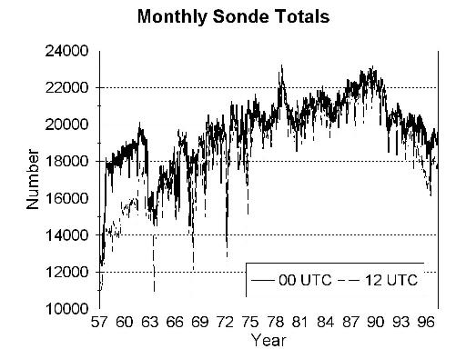
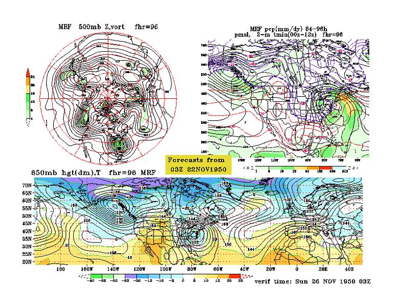
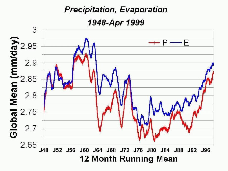